The mesh class

The mesh class holds either geometric definitions (piece-wise linear complex - PLC) or discretizations of the subsurface. It contains of nodes, boundaries (edges in 2D, faces in 3D) and cells (triangles, quadrangles in 2D, hexahedra or tetrahedra in 3D) with associated markers and arbitrary data for nodes or cells.

https://www.pygimli.org/_tutorials_auto/1_basics/plot_2-anatomy_of_a_mesh.html gives a good overview on the properties of a mesh. Here we demonstrate how to create and manipulate meshes from the scratch.

We start off with the typical imports

import numpy as np
import pygimli as pg

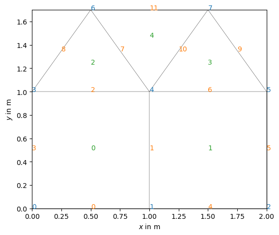
We construct a mesh by creating nodes and cells.

mesh = pg.Mesh(2)  # 2D
n11 = mesh.createNode((0.0, 0.0))
n12 = mesh.createNode((1.0, 0.0))
n13 = mesh.createNode((2.0, 0.0))
n21 = mesh.createNode((0.0, 1.0))
n22 = mesh.createNode((1.0, 1.0), marker=1)
n23 = mesh.createNode((2.0, 1.0))
n31 = mesh.createNode((0.5, 1.7))
n32 = mesh.createNode((1.5, 1.7))
mesh.createQuadrangle(n11, n12, n22, n21, marker=4)
mesh.createQuadrangle(n12, n13, n23, n22, marker=4)
mesh.createTriangle(n21, n22, n31, marker=3)
mesh.createTriangle(n22, n23, n32, marker=3)
mesh.createTriangle(n31, n32, n22, marker=3)  # leave out
print(mesh)

Mesh: Nodes: 8 Cells: 5 Boundaries: 0

The function createNeighborInfos adds boundaries to nodes and cells.

mesh.createNeighborInfos()
print(mesh)

Mesh: Nodes: 8 Cells: 5 Boundaries: 12

We can look only at a given mesh and add matplotlib objects to the plot

ax, _ = pg.show(mesh, showMesh=True)

for n in mesh.nodes():
    ax.text(n.x(), n.y(), str(n.id()), color="C0")
for b in mesh.boundaries():
    ax.text(b.center().x(), b.center().y(), str(b.id()), color="C1")
for c in mesh.cells():
    ax.text(c.center().x(), c.center().y(), str(c.id()), color="C2")

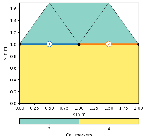
Or we can change and show all (cell or boundary) markers of a mesh

mesh.boundary(2).setMarker(1)
mesh.boundary(6).setMarker(2)
ax, _ = pg.show(mesh, markers=True, showMesh=True)

We can iterate over all nodes, cells, or boundaries and retrieve or change their properties like node positions,

for n in mesh.nodes():
    print(n.id(), n.pos())

0 RVector3: (0.0, 0.0, 0.0)
1 RVector3: (1.0, 0.0, 0.0)
2 RVector3: (2.0, 0.0, 0.0)
3 RVector3: (0.0, 1.0, 0.0)
4 RVector3: (1.0, 1.0, 0.0)
5 RVector3: (2.0, 1.0, 0.0)
6 RVector3: (0.5, 1.7, 0.0)
7 RVector3: (1.5, 1.7, 0.0)

find all nodes of a given cell or find the neighbors,

for c in mesh.cells():
    print(c.id(), len(c.nodes()), c.center())

0 4 RVector3: (0.5, 0.5, 0.0)
1 4 RVector3: (1.5, 0.5, 0.0)
2 3 RVector3: (0.5, 1.2333333333333334, 0.0)
3 3 RVector3: (1.5, 1.2333333333333334, 0.0)
4 3 RVector3: (1.0, 1.4666666666666668, 0.0)

or find the neighboring cells for all inner boundaries.

for b in mesh.boundaries():
    print(b.id(), ": Nodes:", b.ids(), end=" ")
    if not b.outside():
        left = b.leftCell()
        right = b.rightCell()
        print(left.id(), right.id())

0 : Nodes: 2 [0, 1] 1 : Nodes: 2 [1, 4] 0 1
2 : Nodes: 2 [4, 3] 0 2
3 : Nodes: 2 [3, 0] 4 : Nodes: 2 [1, 2] 5 : Nodes: 2 [2, 5] 6 : Nodes: 2 [5, 4] 1 3
7 : Nodes: 2 [4, 6] 2 4
8 : Nodes: 2 [6, 3] 9 : Nodes: 2 [5, 7] 10 : Nodes: 2 [7, 4] 3 4
11 : Nodes: 2 [6, 7]

We visualize some related property and attribute it the mesh cells.

voltage = np.arange(mesh.nodeCount()) + 10
ax, cb = pg.show(mesh, voltage)

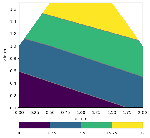
Node-based data are typically shown in form of contour lines.

We can add this (node-based) vector to the mesh as a property. The same can be done for cell-based properties.

mesh["voltage"] = voltage
mesh["velocity"] = np.arange(mesh.cellCount()) + 2
ax, cb = pg.show(mesh, "velocity")

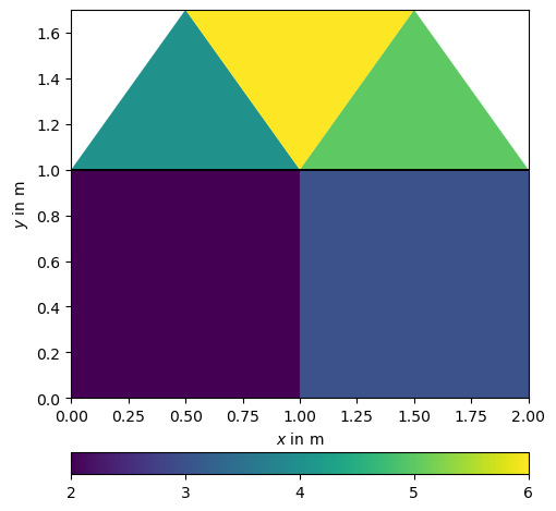
Cell-based data are, on the other hand, valid for the whole cell, which is why they are typically shown by filled patches.

The VTK format can save these properties along with the mesh, point data like the voltage under POINT_DATA and cell data like velocity under CELL_DATA. It is particularly suited to save inversion results in one file. 3D vtk files can be nicely visualized by a number of programs, e.g. Paraview.

if False:
    mesh.exportVTK("mesh.vtk")
    with open("mesh.vtk") as f:
        print(f.read())