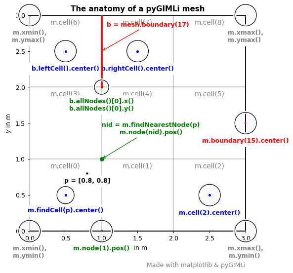
The anatomy of a pyGIMLi mesh

In this tutorial we look at the anatomy of a GIMLI::Mesh. Although the example is simplisitic and two-dimensional, the individual members of the Mesh class and their methods can be inspected similarly for more complex meshes in 2D and 3D. This example is heavily inspired by the anatomy of a matplotlib plot, which we can also highly recommend for visualization with the pygimli.viewer.mpl.

We start by importing matplotlib and defining some helper functions for plotting.

import matplotlib.pyplot as plt

from matplotlib.patches import Circle
from matplotlib.patheffects import withStroke

def circle(x, y, text=None, radius=0.15, c="blue"):
    circle = Circle((x, y), radius, clip_on=False, zorder=10, linewidth=1,
                    edgecolor='black', facecolor=(0, 0, 0, .0125),
                    path_effects=[withStroke(linewidth=5, foreground='w')])
    ax.add_artist(circle)
    ax.plot(x, y, color=c, marker=".")
    ax.text(x, y - (radius + 0.05), text, backgroundcolor="white",
            ha='center', va='top', weight='bold', color=c)

We now import pygimli and create a simple grid/mesh with 3x3 cells.

import pygimli as pg
m = pg.createGrid(4,4)

The following code creates the main plot and shows how the different mesh entities can be called.

# Create matplotlib figure and set size
fig, ax = plt.subplots(figsize=(8,8), dpi=90)
ax.set_title("The anatomy of a pyGIMLi mesh", fontweight="bold")

# Visualize mesh with the generic pg.show command
pg.show(m, ax=ax)

# Number all cells
for cell in m.cells():
    node = cell.allNodes()[2]
    ax.text(node.x() - 0.5, node.y() - .05, "m.cell(%d)" % cell.id(),
            fontsize=11, ha="center", va="top", color="grey")

# Mark horizontal and vertical extent
circle(m.xmin(), m.xmax(), "m.xmin(),\nm.ymax() ", c="grey")
circle(m.xmin(), m.ymin(), "m.xmin(),\nm.ymin() ", c="grey")
circle(m.xmax(), m.ymin(), "m.xmax(),\nm.ymin() ", c="grey")
circle(m.xmax(), m.ymax(), "m.xmax(),\nm.ymax() ", c="grey")

# Mark center of a cell
cid = 2
circle(m.cell(cid).center().x(), m.cell(cid).center().y(),
       "m.cell(%d).center()" % cid)

# Mark node
circle(m.node(1).x(), m.node(1).y(), "m.node(1).pos()", c="green")

# Find cell in which point p lies
p = [0.8, 0.8]
circle(p[0], p[1], "p = %s" % p, radius=0.01, c="black")

cell = m.findCell(p)
circle(cell.center().x(), cell.center().y(), "m.findCell(p).center()",
       radius=0.12)

# Find closest node to point p
nid = m.findNearestNode(p)
n = m.node(nid)
ax.plot(n.x(), n.y(), "go")
ax.annotate('nid = m.findNearestNode(p)\nm.node(nid).pos()', xy=(n.x(), n.y()),
            xycoords='data', xytext=(80, 40), textcoords='offset points',
            ha="center", weight='bold', color="green",
            arrowprops=dict(arrowstyle='->',
                            connectionstyle="arc",
                            color="green"))

# Mark boundary center
bid = 15
boundary_center = m.boundary(bid).center()
circle(boundary_center.x(), boundary_center.y(),
       "m.boundary(%d).center()" % bid, c="red")

# Mark boundary together with left and right cell
bid = 17
b = m.boundaries()[bid] # equivalent to mesh.boundary(17)
n1 = b.allNodes()[0]
n2 = b.allNodes()[1]
ax.plot([n1.x(), n2.x()], [n1.y(), n2.y()], "r-", lw=3, zorder=10)
ax.annotate('b = mesh.boundary(%d)' % bid, xy=(b.center().x(), b.center().y()),
            xycoords='data', xytext=(8, 40), textcoords='offset points',
            weight='bold', color="red",
            arrowprops=dict(arrowstyle='->',
                            connectionstyle="arc",
                            color="red"))
circle(n1.x(), n1.y(), "b.allNodes()[0].x()\nb.allNodes()[0].y()",
       radius=0.1, c="green")

# Mark neighboring cells
left = b.leftCell()
right = b.rightCell()
circle(left.center().x(), left.center().y(),
       "b.leftCell().center()", c="blue")
circle(right.center().x(), right.center().y(),
       "b.rightCell().center()", c="blue")

ax.text(3.0, -0.5, "Made with matplotlib & pyGIMLi",
        fontsize=10, ha="right", color='.5')
fig.tight_layout(pad=5.7)
pg.wait()