VES inversion for a blocky model

This tutorial shows how an built-in forward operator is used for inversion. A DC 1D (VES) modelling is used to generate data, noisify and invert them.

We import numpy, matplotlib and the 1D plotting function

import numpy as np
import matplotlib.pyplot as plt
import pygimli as pg
from pygimli.physics import VESManager

some definitions before (model, data and error)

ab2 = np.logspace(-0.5, 2.5, 40)  # AB/2 distance (current electrodes)

define a synthetic model and do a forward simulatin including noise

synres = [100., 500., 30., 800.]  # synthetic resistivity
synthk = [0.5, 3.5, 6.]  # synthetic thickness (nlay-th layer is infinite)

the forward operator can be called by f.response(model) or simply f(model)

synthModel = synthk + synres  # concatenate thickness and resistivity
ves = VESManager()
rhoa, err = ves.simulate(synthModel, ab2=ab2, mn2=ab2/3,
                         noiseLevel=0.03, seed=1337)

nlay = 4
ves.invert(rhoa, err, ab2=ab2, mn2=ab2/3,
           nLayers=nlay, lam=1000, lambdaFactor=0.8)

7 [0.4862839715507558, 3.1577527561460164, 10.06558804666278, 96.78246471351665, 517.7748284819047, 48.84330357879317, 839.2421863531833]

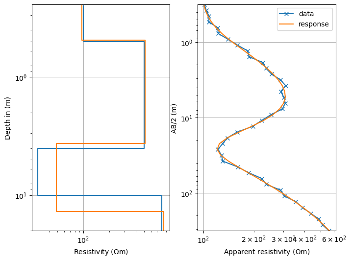
show estimated & synthetic models and data with model response in 2 subplots

fig, ax = plt.subplots(ncols=2, figsize=(8, 6))  # two-column figure
ves.showModel(synthModel, ax=ax[0], label="synth", plot="semilogy", zmax=20)
ves.showModel(ves.model, ax=ax[0], label="model", zmax=20)
ves.showData(rhoa, ax=ax[1], label="data", color="C0", marker="x")
out = ves.showData(ves.inv.response, ax=ax[1], label="response", color="C1")

We are interested in the model uncertaincies and through model covariance

from pygimli.frameworks.resolution import modelCovariance
var, MCM = modelCovariance(ves.inv)
pg.info(var)
fig, ax = plt.subplots()
im = ax.imshow(MCM, vmin=-1, vmax=1, cmap="bwr")
plt.colorbar(im)
labels = [rf'$d_{i+1}$' for i in range(nlay-1)] + \
    [rf'$\rho_{i+1}$' for i in range(nlay)]
plt.xticks(np.arange(nlay*2-1), labels)
_ = plt.yticks(np.arange(nlay*2-1), labels)

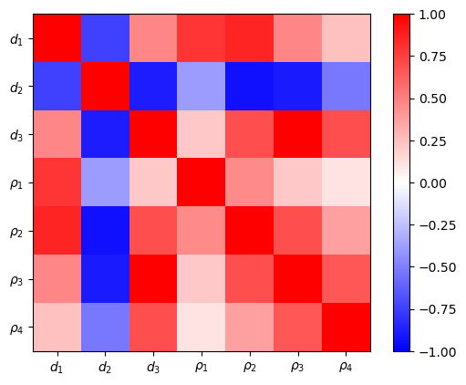
The model covariance matrix delivers variances and a scaled (dimensionless) correlation matrix. The latter show the interdependency of the parameters among each other. The first and last resistivity is best resolved, also the first layer thickness. The remaining resistivities and thicknesses are highly correlated. The variances can be used as error bars in the model plot.

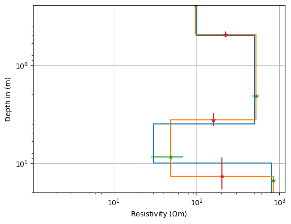
thk = ves.model[:nlay-1]
res = ves.model[nlay-1:]
z = np.cumsum(thk)
mid = np.hstack([z - thk/2, z[-1]*1.1])
resmean = np.sqrt(res[:-1]*res[1:])
fig, ax = plt.subplots()
ves.showModel(synthModel, ax=ax, label="synth", plot="semilogy", zmax=20)
ves.showModel(ves.model, ax=ax, label="model", zmax=20)
ax.errorbar(res, mid, marker="*", ls="None", xerr=res*var[nlay-1:])
_ = ax.errorbar(resmean, z, marker="*", ls="None", yerr=thk*var[:nlay-1])