VES inversion for a smooth model

This tutorial shows how an built-in forward operator is used for an Occam type (smoothness-constrained) inversion with fixed regularization (most natural). A direct current (DC) one-dimensional (1D) VES (vertical electric sounding) modelling operator is used to generate data, add noise and inversion.

We import numpy numerics, mpl plotting, pygimli and the 1D plotting function

import numpy as np
import matplotlib.pyplot as plt

import pygimli as pg
from pygimli.physics.ves import VESRhoModelling, VESManager
from pygimli.viewer.mpl import drawModel1D

Set up synthetic model and simulate data

synRes = [100., 500., 20., 800.]  # synthetic resistivity
synThk = [4, 6, 10]  # synthetic thickness (lay layer is infinite)
ab2 = np.logspace(-1, 2, 25)  # 0.1 to 100 in 25 steps (8 points per decade)
ves = VESManager()
rhoa, error = ves.simulate(synThk+synRes, ab2=ab2, mn2=ab2/3,
                           noiseLevel=0.03, seed=1337)

Set up the forward operator

thk = np.logspace(-0.5, 0.5, 30)
f = VESRhoModelling(thk=thk, ab2=ab2, mn2=ab2/3)

Set up inversion

inv = pg.Inversion(fop=f, verbose=False)
# inv.setRegularization(cType=1)  # default = not necessary

Create some transformations used for inversion

inv.transData = pg.trans.TransLog()  # log transformation also for data
inv.transModel = pg.trans.TransLogLU(1, 1000)  # lower and upper bound

Set pretty large regularization strength and run inversion

print("inversion with lam=100")
res100 = inv.run(rhoa, error, lam=100)
print('rrms={:.2f}%, chi^2={:.3f}'.format(inv.relrms(), inv.chi2()))

inversion with lam=100
rrms=5.15%, chi^2=2.951

Decrease the regularization (smoothness) and repeat

print("inversion with lam=10")
res10 = inv.run(rhoa, error, lam=10)
print('rrms={:.2f}%, chi^2={:.3f}'.format(inv.relrms(), inv.chi2()))

inversion with lam=10
rrms=3.43%, chi^2=1.309

Decrease the regularization (smoothness) and repeat

print("inversion with second order smoothness")
inv.setRegularization(cType=2)
resC2 = inv.run(rhoa, error, lam=20)
print('rrms={:.2f}%, chi^2={:.3f}'.format(inv.relrms(), inv.chi2()))

inversion with second order smoothness
rrms=3.06%, chi^2=1.038

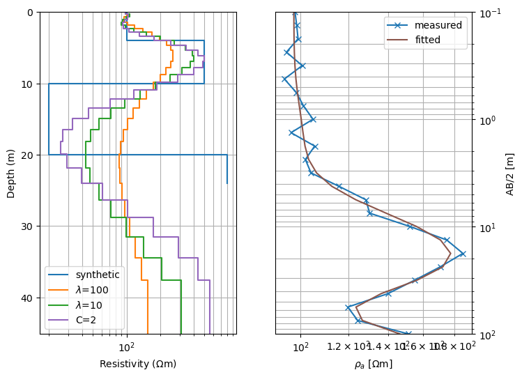
Show model (inverted and synthetic) as well as model response and data

fig, ax = plt.subplots(ncols=2, figsize=(8, 6))  # two-column figure
drawModel1D(ax[0], synThk, synRes, color='C0', label='synthetic',
            plot='semilogx')
drawModel1D(ax[0], thk, res100, color='C1', label=r'$\lambda$=100')
drawModel1D(ax[0], thk, res10, color='C2', label=r'$\lambda$=10')
drawModel1D(ax[0], thk, resC2, color='C4', label=r'C=2')
ax[0].grid(True, which='both')
ax[0].legend(loc='best')
ax[1].loglog(rhoa, ab2, 'x-', color="C0", label='measured')
ax[1].loglog(inv.response, ab2, '-', color="C5", label='fitted')
ax[1].set_ylim((max(ab2), min(ab2)))
ax[1].grid(True, which='both')
ax[1].set_xlabel(r'$\rho_a$ [$\Omega$m]')
ax[1].set_ylabel('AB/2 [m]')
ax[1].yaxis.set_label_position('right')
ax[1].yaxis.set_ticks_position('right')
ax[1].legend(loc='best');

<matplotlib.legend.Legend object at 0x329c49d00>