pygimli.viewer.mpl#
Drawing functions using Matplotlib.
Overview#
Functions
|
Add alpha values to the colors of a polygon collection. |
|
Set some common default properties for an axe. |
|
Create nLevs bins for the data array z based on matplotlib ticker. |
|
Get a colormap either from name or from keyworld list. |
|
Create animation for the content of a given matplotlib figure. |
|
Create a Colorbar. |
|
Create figure with a colorbar. |
|
Utility function to create 2d mesh patches within a given ax. |
|
Generate triangle objects for later drawing. |
|
Utility function to create (or return existing) twin x axes for ax. |
|
Utility function to create (or return existing) twin x axes for ax. |
|
Create a list of patch objects that can be used for borehole legends. |
|
Draw a 1D column (e.g., from a 1D inversion) on a given ax. |
|
DEPRECATED. |
|
Draw a view of a matrix into the axes. |
|
Draw boundary markers for mesh.boundaries with marker != 0 |
|
Draw previously generated (generateVecMatrix) matrix. |
|
Draw mesh with scalar field data. |
|
Draw a 2d mesh into a given ax. |
|
Draw mesh on ax with boundary conditions colorized. |
|
Draw a 2d mesh and color the cell by the data. |
|
Draw 1d block model into axis ax. |
|
Draw 2D PLC into given axes. |
|
Draw inter parameter constraints between cells. |
|
Draw mesh boundaries into a given axes. |
|
Draw mesh boundaries as shadows into a given axes. |
|
Draw Sensor marker, these marker are pickable. |
|
Draw sensor positions as black dots with a given diameter. |
|
Draw a view of a matrix into the axes. |
|
Draw streamlines for the gradients of field values u on a mesh. |
|
Draw streamlines based on an unstructured mesh. |
|
Show values as patches over x and y vector. |
|
Draw x, y, v vectors in form of a matrix. |
|
TODO Documentme. |
|
Generate a data matrix from x/y and value vectors. |
|
TODO WRITEME. |
|
Replace the last-but-one tick label by unit symbol. |
Returns False if a non-interactive backend is used, e.g. for Jupyter Notebooks and sphinx builds. |
|
|
Toggle quiet mode to avoid popping figures. |
|
Plot previously generated (generateVecMatrix) matrix. |
|
Plot previously generated (generateVecMatrix) y map (category). |
|
Plot datacontainer as matrix (deprecated). |
|
Read lines from file and plot over model. |
|
Naming conventions. |
|
Plot vectors as matrix (deprecated). |
If called it register a closing function that will ensure all pending MPL figures are shown. |
|
|
Switch signs of depth ticks to be positive |
|
Create and save an animation for a given mesh with a set of field data. |
|
Save axes as pdf. |
|
Save figure as pdf. |
|
Set colorbar levels given a number of levels and min/max values. |
|
Change the data values for a given mappable. |
|
Set preferred output style. |
|
TODO merge with setOutputStyle. |
|
Show 1d block model defined by value and thickness vectors. |
|
Plot data container as matrix (cross-plot). |
|
Show value map as matrix. |
|
Show several 1d block models as (stitched) section. |
|
Show values as patches over x and y vector. |
|
Plot three vectors as matrix. |
|
Show FDEM sounding as real(inphase) and imaginary (quadrature) fields. |
|
Return the twin of ax if exist. |
|
For internal use. |
|
Update colorbar values. |
|
For internal use. |
|
TODO WRITEME. |
Classes
|
Class for handling (structural) borehole data for inclusion in plots. |
|
Class to load and handle several boreholes belonging to one profile. |
|
Interactive cell browser on current or specified ax for a given mesh. |
Functions#
- pygimli.viewer.mpl.addCoverageAlpha(patches, coverage, dropThreshold=0.4)[source]#
Add alpha values to the colors of a polygon collection.
- Parameters:
patches (2D mpl mappable)
coverage (array) – coverage values. Maximum coverage mean no opaqueness.
dropThreshold (float) – relative minimum coverage
- pygimli.viewer.mpl.adjustWorldAxes(ax, useDepth: bool = True, xl: str = '$x$ in m', yl: str = None)[source]#
Set some common default properties for an axe.
- pygimli.viewer.mpl.autolevel(z, nLevs, logScale=None, zMin=None, zMax=None)[source]#
Create nLevs bins for the data array z based on matplotlib ticker.
Examples
>>> import numpy as np
>>> from pygimli.viewer.mpl import autolevel
>>> x = np.linspace(1, 10, 100)
>>> autolevel(x, 3)
array([ 1. ,  5.5, 10. ])
>>> x = np.linspace(1, 1000, 100)
>>> autolevel(x, 4, logScale=True)
array([   1.,   10.,  100., 1000.])
- pygimli.viewer.mpl.cmapFromName(cmapname='jet', ncols=256, bad=None, **kwargs)[source]#
Get a colormap either from name or from keyworld list.
See http://matplotlib.org/examples/color/colormaps_reference.html
- pygimli.viewer.mpl.createAnimation(fig, animate, nFrames, dpi, out)[source]#
Create animation for the content of a given matplotlib figure.
Until I know a better place.
- pygimli.viewer.mpl.createColorBar(gci, orientation='horizontal', size=0.2, pad=None, **kwargs)[source]#
Create a Colorbar.
Shortcut to create a matplotlib colorbar within the ax for a given patchset. The colorbar is stored in the axes object as __cBar__ to avoid duplicates.
- pygimli.viewer.mpl.createColorBarOnly(cMin=1, cMax=100, logScale=False, cMap=None, nLevs=5, label=None, orientation='horizontal', savefig=None, ax=None, **kwargs)[source]#
Create figure with a colorbar.
- Parameters:
**kwargs – Forwarded to mpl.colorbar.ColorbarBase.
- Returns:
The created figure.
- Return type:
fig
Examples
>>> # import pygimli as pg
>>> # from pygimli.viewer.mpl import createColorBarOnly
>>> # createColorBarOnly(cMin=0.2, cMax=5, logScale=False,
>>> #                   cMap='b2r',
>>> #                   nLevs=7,
>>> #                   label=r'Ratio',
>>> #                   orientation='horizontal')
>>> # pg.wait()
Examples using pygimli.viewer.mpl.createColorBarOnly
- pygimli.viewer.mpl.createMeshPatches(ax, mesh, rasterized=False, verbose=True)[source]#
Utility function to create 2d mesh patches within a given ax.
- pygimli.viewer.mpl.createTriangles(mesh)[source]#
Generate triangle objects for later drawing.
Creates triangle for each 2D triangle cell or 3D boundary. Quads will be split into two triangles. Result will be cached into mesh._triData.
- Parameters:
mesh (GIMLI::Mesh) – 2D mesh or 3D mesh
- Returns:
x (numpy array) – x position of nodes
y (numpy array) – x position of nodes
triangles (numpy array Cx3) – cell indices for each triangle, quad or boundary face
z (numpy array) – z position for given indices
dataIdx (list of int) – List of indices for a data array
- pygimli.viewer.mpl.createTwinX(ax)[source]#
Utility function to create (or return existing) twin x axes for ax.
- pygimli.viewer.mpl.createTwinY(ax)[source]#
Utility function to create (or return existing) twin x axes for ax.
- pygimli.viewer.mpl.create_legend(ax, cmap, ids, classes)[source]#
Create a list of patch objects that can be used for borehole legends.
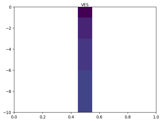
- pygimli.viewer.mpl.draw1DColumn(ax, x, val, thk, width=30, ztopo=0, cMin=1, cMax=1000, cMap=None, name=None, textoffset=0.0, **kwargs)[source]#
Draw a 1D column (e.g., from a 1D inversion) on a given ax.
Examples
>>> import numpy as np
>>> import matplotlib.pyplot as plt
>>> from pygimli.viewer.mpl import draw1DColumn
>>> thk = [1, 2, 3, 4]
>>> val = thk
>>> fig, ax = plt.subplots()
>>> draw1DColumn(ax, 0.5, val, thk, width=0.1, cmin=1, cmax=4, name="VES")
<matplotlib.collections.PatchCollection object at ...>
>>> _ = ax.set_ylim(-np.sum(thk), 0)

Examples using pygimli.viewer.mpl.draw1DColumn
- pygimli.viewer.mpl.draw1dmodel(x, thk=None, xlab=None, zlab='z in m', islog=True, z0=0)[source]#
DEPRECATED.
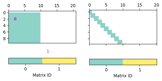
- pygimli.viewer.mpl.drawBlockMatrix(ax, mat, **kwargs)[source]#
Draw a view of a matrix into the axes.
- Parameters:
ax (mpl axis instance, optional) – Axis instance where the matrix will be plotted.
mat (pg.Matrix.BlockMatrix)
- Keyword Arguments:
spy (bool [False]) – Draw all matrix entries instead of colored blocks
- Return type:
ax
Examples
>>> import numpy as np
>>> import pygimli as pg
>>> I = pg.matrix.IdentityMatrix(10)
>>> SM = pg.matrix.SparseMapMatrix()
>>> for i in range(10):
...     SM.setVal(i, 10 - i, 5.0)
...     SM.setVal(i,  i, 5.0)
>>> B = pg.matrix.BlockMatrix()
>>> B.add(I, 0, 0)
0
>>> B.add(SM, 10, 10)
1
>>> print(B)
pg.matrix.BlockMatrix of size 20 x 21 consisting of 2 submatrices.
>>> fig, (ax1, ax2) = pg.plt.subplots(1, 2, sharey=True)
>>> _ = pg.show(B, ax=ax1)
>>> _ = pg.show(B, spy=True, ax=ax2)

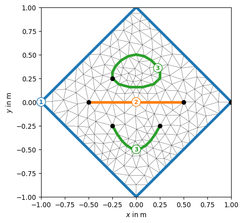
- pygimli.viewer.mpl.drawBoundaryMarkers(ax, mesh, clipBoundaryMarkers=False, **kwargs)[source]#
Draw boundary markers for mesh.boundaries with marker != 0
- Parameters:
mesh (GIMLI::Mesh) – Mesh that have the boundary markers.
clipBoundaryMarkers (bool [False]) – Clip boundary marker to the axes limits if needed.
- Keyword Arguments:
**kwargs – Forwarded to plot
Examples
>>> import pygimli as pg
>>> import pygimli.meshtools as mt
>>> c0 = mt.createCircle(pos=(0.0, 0.0), radius=1, nSegments=4)
>>> l0 = mt.createPolygon([[-0.5, 0.0], [.5, 0.0]], boundaryMarker=2)
>>> l1 = mt.createPolygon([[-0.25, -0.25], [0.0, -0.5], [0.25, -0.25]],
...                       interpolate='spline', addNodes=4,
...                       boundaryMarker=3)
>>> l2 = mt.createPolygon([[-0.25, 0.25], [0.0, 0.5], [0.25, 0.25]],
...                       interpolate='spline', addNodes=4,
...                       isClosed=True, boundaryMarker=3)
>>> mesh = mt.createMesh([c0, l0, l1, l2], area=0.01)
>>> ax, _ = pg.show(mesh)
>>> pg.viewer.mpl.drawBoundaryMarkers(ax, mesh)

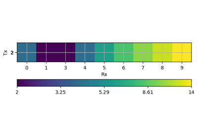
- pygimli.viewer.mpl.drawDataMatrix(ax, mat, xmap=None, ymap=None, cMin=None, cMax=None, logScale=None, label=None, **kwargs)[source]#
Draw previously generated (generateVecMatrix) matrix.
- Parameters:
ax (mpl.axis) – axis to plot, if not given a new figure is created
mat (numpy.array2d) – matrix to show
xmap (dict {i:num}) – dict (must match A.shape[0])
ymap (iterable) – vector for x axis (must match A.shape[0])
cMin/cMax (float) – minimum/maximum color values
logScale (bool) – logarithmic colour scale [min(A)>0]
label (string) – colorbar label
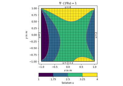
- pygimli.viewer.mpl.drawField(ax, mesh, data=None, levels=None, nLevs=5, cMin=None, cMax=None, nCols=None, logScale=False, fitView=True, **kwargs)[source]#
Draw mesh with scalar field data.
Draw scalar field into MPL axes using matplotlib triplot. Only for triangle/quadrangle meshes currently
- Parameters:
ax (Matplotlib axis object)
mesh (GIMLI::Mesh) – 2D mesh
data (iterable) – Scalar field values. Can be of length mesh.cellCount() or mesh.nodeCount().
levels (iterable of type float) – Values for contour lines. If empty auto generated from nLevs.
nLevs (int) – Number of contour levels based on cMin, cMax and logScale.
cMin (float [None]) – Minimal contour value. If None min(data).
cMax (float [None]) – Maximal contour value. If None max(data).
logScale (bool [False]) – Levels and colors distributes with logarithmic scale.
fitView (bool [True]) – Adjust ax limits to mesh bounding box.
- Keyword Arguments:
shading ('flat' | 'gouraud')
fillContour ([True])
contourLines ([True])
**kwargs – Additional kwargs forwarded to ax.tripcolor, ax.tricontour, ax.tricontourf
- Returns:
gci – The current image object useful for post color scaling
- Return type:
image object
Examples
>>> import numpy as np
>>> import matplotlib.pyplot as plt
>>> import pygimli as pg
>>> from pygimli.viewer.mpl import drawField
>>> n = np.linspace(0, -2, 11)
>>> mesh = pg.createGrid(x=n, y=n)
>>> nx = pg.x(mesh.positions())
>>> ny = pg.y(mesh.positions())
>>> data = np.cos(1.5 * nx) * np.sin(1.5 * ny)
>>> fig, ax = plt.subplots()
>>> tri = drawField(ax, mesh, data)
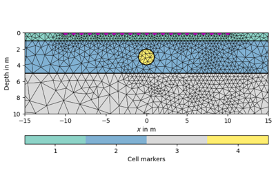
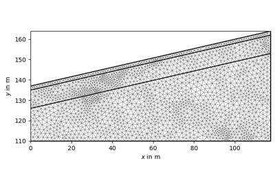
- pygimli.viewer.mpl.drawMesh(ax, mesh, fitView=True, **kwargs)[source]#
Draw a 2d mesh into a given ax.
Set the limits of the ax tor the mesh extent.
- Parameters:
ax (mpl axe instance) – Axis instance where the mesh is plotted.
mesh (GIMLI::Mesh) – The 2D mesh which will be drawn.
fitView (bool [True]) – Adjust ax limits to mesh bounding box.
- Keyword Arguments:
**kwargs – Additional kwargs forward to drawPLC or drawMeshBoundaries.
%(drawMeshBoundaries)
%(drawPLC)
Examples
>>> import numpy as np
>>> import matplotlib.pyplot as plt
>>> import pygimli as pg
>>> from pygimli.viewer.mpl import drawMesh
>>> n = np.linspace(1, 2, 10)
>>> mesh = pg.createGrid(x=n, y=n)
>>> fig, ax = plt.subplots()
>>> drawMesh(ax, mesh)
>>> plt.show()
Examples using pygimli.viewer.mpl.drawMesh
- pygimli.viewer.mpl.drawMeshBoundaries(ax, mesh, hideMesh=False, useColorMap=False, fitView=True, lw=None, color=None, **kwargs)[source]#
Draw mesh on ax with boundary conditions colorized.
- Parameters:
mesh (GIMLI::Mesh)
hideMesh (bool [False]) – Show only the boundary of the mesh and omit inner edges that separate the cells.
useColorMap (bool[False]) – Apply the default colormap to boundaries with marker values > 0
fitView (bool [True]) – Adjust ax limits to mesh bounding box.
lw (float [None]) – Linewidth. When set to None then lw depends on boundary marker. Linewidth [0.3] for edges with marker == 0 if hideMesh is False.
color (None) – Color for special lines. If set to None automatic “black”.
Examples
>>> import numpy as np
>>> import matplotlib.pyplot as plt
>>> import pygimli as pg
>>> from pygimli.viewer.mpl import drawMeshBoundaries
>>> n = np.linspace(0, -2, 11)
>>> mesh = pg.createGrid(x=n, y=n)
>>> for bound in mesh.boundaries():
...     if not bound.rightCell():
...         bound.setMarker(pg.core.MARKER_BOUND_MIXED)
...     if bound.center().y() == 0:
...         bound.setMarker(pg.core.MARKER_BOUND_HOMOGEN_NEUMANN)
>>> fig, ax = plt.subplots()
>>> drawMeshBoundaries(ax, mesh)

- pygimli.viewer.mpl.drawModel(ax, mesh, data=None, tri=False, rasterized=False, cMin=None, cMax=None, logScale=False, xlabel=None, ylabel=None, fitView=True, verbose=False, **kwargs)[source]#
Draw a 2d mesh and color the cell by the data.
- Parameters:
ax (mpl axis instance, optional) – Axis instance where the mesh is plotted (default is current axis).
mesh (GIMLI::Mesh) – The plotted mesh to browse through.
data (array, optional) – Data to draw. Should either equal numbers of cells or nodes of the corresponding mesh.
tri (boolean, optional) – use MPL tripcolor (experimental)
rasterized (boolean, optional) – Rasterize mesh patches to reduce file size and avoid zooming artifacts in some PDF viewers.
fitView (bool [True]) – Adjust ax limits to mesh bounding box.
- Keyword Arguments:
**kwargs – Additional kwargs forwarded to the draw functions and mpl methods, respectively.
- Returns:
gci
- Return type:
matplotlib graphics object
Examples
>>> import numpy as np
>>> import matplotlib.pyplot as plt
>>> import pygimli as pg
>>> from pygimli.viewer.mpl import drawModel
>>> n = np.linspace(0, -2, 11)
>>> mesh = pg.createGrid(x=n, y=n)
>>> mx = pg.x(mesh.cellCenter())
>>> my = pg.y(mesh.cellCenter())
>>> data = np.cos(1.5 * mx) * np.sin(1.5 * my)
>>> fig, ax = plt.subplots()
>>> drawModel(ax, mesh, data)
<matplotlib.collections.PolyCollection object at ...>
Examples using pygimli.viewer.mpl.drawModel
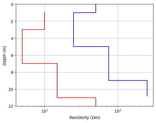
- pygimli.viewer.mpl.drawModel1D(ax, thickness=None, values=None, model=None, depths=None, plot='plot', xlabel='Resistivity $(\\Omega$m$)$', zlabel='Depth (m)', z0=0, zmax=None, **kwargs)[source]#
Draw 1d block model into axis ax.
Draw 1d block model into axis ax defined by values and thickness vectors using plot function. For log y cases, z0 should be set > 0 so that the default becomes 1.
- Parameters:
ax (mpl axes) – Matplotlib Axes object to plot into.
values (iterable [float]) – [N] Values for each layer plus lower background.
thickness (iterable [float]) – [N-1] thickness for each layer. Either thickness or depths must be set.
depths (iterable [float]) – [N-1] Values for layer depths (positive z-coordinates). Either thickness or depths must be set.
model (iterable [float]) – Shortcut to use default model definition. thks = model[0:nLay] values = model[nLay:]
plot (string) – Matplotlib plotting function. ‘plot’, ‘semilogx’, ‘semilogy’, ‘loglog’
xlabel (str) – Label for x axis.
ylabel (str) – Label for y axis.
z0 (float) – Starting depth in m
**kwargs (dict()) – Forwarded to the plot routine
Examples
>>> import matplotlib.pyplot as plt
>>> import numpy as np
>>> import pygimli as pg
>>> # plt.style.use('ggplot')
>>> thk = [1, 4, 4]
>>> res = np.array([10., 5, 15, 50])
>>> fig, ax = plt.subplots()
>>> pg.viewer.mpl.drawModel1D(ax, values=res*5, depths=np.cumsum(thk),
...                          plot='semilogx', color='blue')
>>> pg.viewer.mpl.drawModel1D(ax, values=res, thickness=thk, z0=1,
...                          plot='semilogx', color='red')
>>> pg.wait()
Examples using pygimli.viewer.mpl.drawModel1D
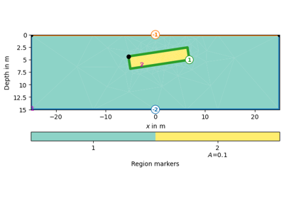
- pygimli.viewer.mpl.drawPLC(ax, mesh, fillRegion=True, regionMarker=True, boundaryMarkers=False, showNodes=False, fitView=True, **kwargs)[source]#
Draw 2D PLC into given axes.
- Parameters:
ax (mpl axe)
mesh (GIMLI::Mesh)
fillRegion (bool [True]) – Fill the regions with default colormap.
regionMarker (bool [True]) – Show region marker.
boundaryMarkers (bool [False]) – Show boundary marker.
showNodes (bool [False]) – Draw all nodes as little dots.
fitView (bool [True]) – Adjust ax limits to mesh bounding box.
- Keyword Arguments:
**kwargs – Additional kwargs forwarded to the draw functions and mpl methods, respectively.
Examples
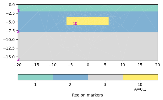
>>> import matplotlib.pyplot as plt
>>> import pygimli as pg
>>> import pygimli.meshtools as mt
>>> # Create geometry definition for the modelling domain
>>> world = mt.createWorld(start=[-20, 0], end=[20, -16],
...                        layers=[-2, -8], worldMarker=False)
>>> # Create a heterogeneous block
>>> block = mt.createRectangle(start=[-6, -3.5], end=[6, -6.0],
...                            marker=10,  boundaryMarker=10, area=0.1)
>>> fig, ax = plt.subplots()
>>> geom = world + block
>>> _ = pg.viewer.mpl.drawPLC(ax, geom)
Examples using pygimli.viewer.mpl.drawPLC
- pygimli.viewer.mpl.drawParameterConstraints(ax, mesh, cMat, cWeights=None)[source]#
Draw inter parameter constraints between cells.
- Parameters:
ax (MPL axes)
mesh (GIMLI::Mesh) – 2d mesh
cMat (GIMLI::SparseMapMatrix) – ConstraintsMatrix
cWeights (iterable float) – Weights for all constraints. Need to have a lengths == cMat.rows()
- pygimli.viewer.mpl.drawSelectedMeshBoundaries(ax, boundaries, color=None, linewidth=1.0, linestyle='-', **kwargs)[source]#
Draw mesh boundaries into a given axes.
- Parameters:
ax (matplotlib axes) – axes to plot into
boundaries (GIMLI::Mesh boundary vector) – collection of boundaries to plot
color (matplotlib color |str [None]) – matching color or string, else colors are according to markers
linewidth (float [1.0]) – line width
linestyles (linestyle for line collection, i.e. solid or dashed)
- Returns:
lco
- Return type:
matplotlib line collection object
- pygimli.viewer.mpl.drawSelectedMeshBoundariesShadow(ax, boundaries, first='x', second='y', color=(0.3, 0.3, 0.3, 1.0))[source]#
Draw mesh boundaries as shadows into a given axes.
- Parameters:
ax (matplotlib axes) – axes to plot into
boundaries (GIMLI::Mesh boundary vector) – collection of boundaries to plot
second (first /) – attribute names to retrieve from nodes
color (matplotlib color |str [None]) – matching color or string, else colors are according to markers
linewidth (float [1.0]) – line width
- Returns:
lco
- Return type:
matplotlib line collection object
- pygimli.viewer.mpl.drawSensorAsMarker(ax, data)[source]#
Draw Sensor marker, these marker are pickable.
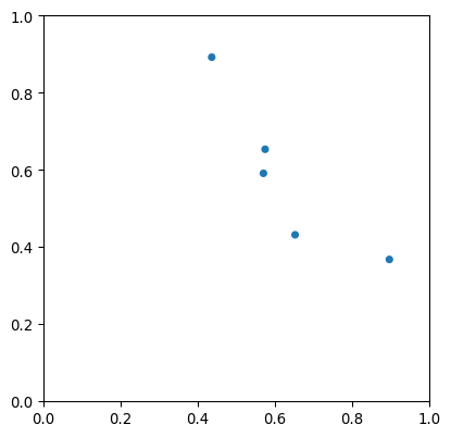
- pygimli.viewer.mpl.drawSensors(ax, sensors, diam=None, coords=None, **kwargs)[source]#
Draw sensor positions as black dots with a given diameter.
- Parameters:
- Keyword Arguments:
**kwargs – Additional kwargs forwarded to mpl.PatchCollection, mpl.Circle
sensorMarker – Also ‘sm’. Set marker style: ‘o’ Circle, ‘v’ Triangle pointing down.
Examples
>>> import numpy as np
>>> import matplotlib.pyplot as plt
>>> import pygimli as pg
>>> from pygimli.viewer.mpl import drawSensors
>>> sensors = np.random.rand(5, 2)
>>> fig, ax = pg.plt.subplots()
>>> drawSensors(ax, sensors, diam=0.02, coords=[0, 1])
>>> ax.set_aspect('equal')
>>> pg.wait()
Examples using pygimli.viewer.mpl.drawSensors
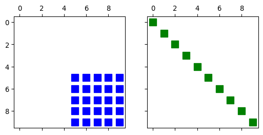
- pygimli.viewer.mpl.drawSparseMatrix(ax, mat, **kwargs)[source]#
Draw a view of a matrix into the axes.
- Parameters:
ax (mpl axis instance, optional) – Axis instance where the matrix will be plotted.
mat (pg.matrix.SparseMatrix or pg.matrix.SparseMapMatrix)
- Return type:
mpl.lines.line2d
Examples
>>> import numpy as np
>>> import pygimli as pg
>>> from pygimli.viewer.mpl import drawSparseMatrix
>>> A = pg.randn((10,10), seed=0)
>>> SM = pg.matrix.SparseMapMatrix()
>>> for i in range(10):
...     SM.setVal(i, i, 5.0)
>>> fig, (ax1, ax2) = pg.plt.subplots(1, 2, sharey=True, sharex=True)
>>> _ = drawSparseMatrix(ax1, A, colOffset=5, rowOffset=5, color='blue')
>>> _ = drawSparseMatrix(ax2, SM, color='green')
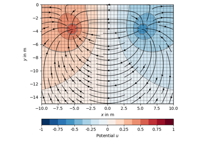
- pygimli.viewer.mpl.drawStreamLines(ax, mesh, u, nx=25, ny=25, **kwargs)[source]#
Draw streamlines for the gradients of field values u on a mesh.
The matplotlib routine streamplot needs equidistant spacings so we interpolate first on a grid defined by nx and ny nodes. Additionally arguments are piped to streamplot.
This works only for rectangular regions. You should use pg.viewer.mpl.drawStreams, which is more comfortable and more flexible.
- Parameters:
ax (mpl axe)
mesh (GIMLI::Mesh) – 2D mesh
u (iterable float) – Scalar data field.
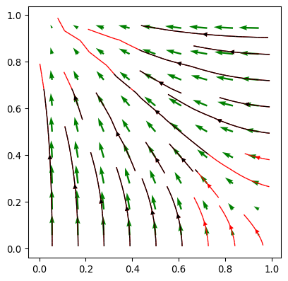
- pygimli.viewer.mpl.drawStreams(ax, mesh, data, startStream=3, coarseMesh=None, quiver=False, **kwargs)[source]#
Draw streamlines based on an unstructured mesh.
Every cell contains only one streamline and every new stream line starts in the center of a cell. You can alternatively provide a second mesh with coarser mesh to draw streams for.
- Parameters:
ax (matplotlib.ax) – ax to draw into
mesh (GIMLI::Mesh) – 2d mesh
data (iterable float | [float, float] | pg.PosVector) – If data is an array (per cell or node) gradients are calculated otherwise the data will be interpreted as vector field per nodes or cell centers.
startStream (int) – variate the start stream drawing, try values from 1 to 3 what every you like more.
coarseMesh (GIMLI::Mesh) – Instead of draw a stream for every cell in mesh, draw a streamline segment for each cell in coarseMesh.
quiver (bool [False]) – Draw arrows instead of streamlines.
- Keyword Arguments:
**kwargs – Additional kwargs forwarded to axe.quiver, drawStreamLine
Examples
>>> import numpy as np
>>> import matplotlib.pyplot as plt
>>> import pygimli as pg
>>> from pygimli.viewer.mpl import drawStreams
>>> n = np.linspace(0, 1, 10)
>>> mesh = pg.createGrid(x=n, y=n)
>>> nx = pg.x(mesh.positions())
>>> ny = pg.y(mesh.positions())
>>> data = np.cos(1.5 * nx) * np.sin(1.5 * ny)
>>> fig, ax = plt.subplots()
>>> drawStreams(ax, mesh, data, color='red')
>>> drawStreams(ax, mesh, data, dropTol=0.9)
>>> drawStreams(ax, mesh, pg.solver.grad(mesh, data),
...             color='green', quiver=True)
>>> ax.set_aspect('equal')
>>> pg.wait()
Examples using pygimli.viewer.mpl.drawStreams
- pygimli.viewer.mpl.drawValMapPatches(ax, vals, xVec=None, yVec=None, dx=1, dy=None, **kwargs)[source]#
Show values as patches over x and y vector.
- pygimli.viewer.mpl.drawVecMatrix(ax, xvec, yvec, vals, full=False, **kwargs)[source]#
Draw x, y, v vectors in form of a matrix.
- pygimli.viewer.mpl.findAndMaskBestClim(dataIn, cMin=None, cMax=None, dropColLimitsPerc=5, logScale=False)[source]#
TODO Documentme.
- pygimli.viewer.mpl.generateMatrix(xvec, yvec, vals, **kwargs)[source]#
Generate a data matrix from x/y and value vectors.
- Parameters:
xvec (iterables (list, np.array, pg.Vector) of same length)
yvec (iterables (list, np.array, pg.Vector) of same length)
vals (iterables (list, np.array, pg.Vector) of same length)
full (bool [False]) – generate a fully symmetric matrix containing all unique xvec+yvec otherwise A is squeezed to the individual unique vectors
- Returns:
A (np.ndarray(2d)) – matrix containing the values sorted according to unique xvec/yvec
xmap/ymap (dict {key: num}) – dictionaries for accessing matrix position (row/col number from x/y[i])
- pygimli.viewer.mpl.insertUnitAtNextLastTick(ax, unit, xlabel=True, position=-2)[source]#
Replace the last-but-one tick label by unit symbol.
- pygimli.viewer.mpl.isInteractive()[source]#
Returns False if a non-interactive backend is used, e.g. for Jupyter Notebooks and sphinx builds.
- pygimli.viewer.mpl.noShow(on=True)[source]#
Toggle quiet mode to avoid popping figures.
- Parameters:
on (bool[True]) – Set Matplotlib backend to ‘agg’ and restore old backend if set to False.
- pygimli.viewer.mpl.patchMatrix(mat, xmap=None, ymap=None, ax=None, cMin=None, cMax=None, logScale=None, label=None, dx=1, **kwargs)[source]#
Plot previously generated (generateVecMatrix) matrix.
- Parameters:
mat (numpy.array2d) – matrix to show
xmap (dict {i:num}) – dict (must match A.shape[0])
ymap (iterable) – vector for x axis (must match A.shape[0])
ax (mpl.axis) – axis to plot, if not given a new figure is created
cMin/cMax (float) – minimum/maximum color values
logScale (bool) – logarithmic colour scale [min(A)>0]
label (string) – colorbar label
dx (float) – width of the matrix elements (by default 1)
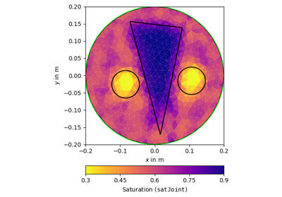
- pygimli.viewer.mpl.patchValMap(vals, xvec=None, yvec=None, ax=None, cMin=None, cMax=None, logScale=None, label=None, dx=1, dy=None, cTrim=0, **kwargs)[source]#
Plot previously generated (generateVecMatrix) y map (category).
- Parameters:
vals (iterable) – Data values to show.
xvec (dict {i:num}) – dict (must match vals.shape[0])
ymap (iterable) – vector for x axis (must match vals.shape[0])
ax (mpl.axis) – axis to plot, if not given a new figure is created
cMin/cMax (float) – minimum/maximum color values
cTrim (float [0]) – use trim value to exclude outer cTrim percent of data from color scale
logScale (bool) – logarithmic colour scale [min(vals)>0]
label (string) – colorbar label
kwargs (**) –
- circularbool
Plot in polar coordinates.
- pygimli.viewer.mpl.plotDataContainerAsMatrix(*args, **kwargs)[source]#
Plot datacontainer as matrix (deprecated).
- pygimli.viewer.mpl.plotLines(ax, line_filename, linewidth=1.0, step=1)[source]#
Read lines from file and plot over model.
- pygimli.viewer.mpl.plotMatrix(mat, *args, **kwargs)[source]#
Naming conventions. Use drawDataMatrix or showDataMatrix instead.
- pygimli.viewer.mpl.plotVecMatrix(xvec, yvec, vals, full=False, **kwargs)[source]#
Plot vectors as matrix (deprecated).
- pygimli.viewer.mpl.registerShowPendingFigsAtExit()[source]#
If called it register a closing function that will ensure all pending MPL figures are shown.
Its only set on demand by pg.show() since we only need it if matplotlib is used.
- pygimli.viewer.mpl.saveAnimation(mesh, data, out, vData=None, plc=None, label='', cMin=None, cMax=None, logScale=False, cmap=None, **kwargs)[source]#
Create and save an animation for a given mesh with a set of field data.
Until I know a better place.
- pygimli.viewer.mpl.setCbarLevels(cbar, cMin=None, cMax=None, nLevs=5, levels=None)[source]#
Set colorbar levels given a number of levels and min/max values.
- pygimli.viewer.mpl.setMappableData(mappable, dataIn, cMin=None, cMax=None, logScale=None, **kwargs)[source]#
Change the data values for a given mappable.
- pygimli.viewer.mpl.setOutputStyle(dim='w', paperMargin=5, xScale=1.0, yScale=1.0, fontsize=9, scale=1, usetex=True)[source]#
Set preferred output style.
- pygimli.viewer.mpl.setPlotStuff(fontsize=7, dpi=None)[source]#
TODO merge with setOutputStyle.
Change ugly name.
- pygimli.viewer.mpl.show1dmodel(x, thk=None, xlab=None, zlab='z in m', islog=True, z0=0, **kwargs)[source]#
Show 1d block model defined by value and thickness vectors.
- pygimli.viewer.mpl.showDataContainerAsMatrix(data, x=None, y=None, v=None, **kwargs)[source]#
Plot data container as matrix (cross-plot).
for each x, y and v token strings or vectors should be given
Examples using pygimli.viewer.mpl.showDataContainerAsMatrix
- pygimli.viewer.mpl.showDataMatrix(mat, xmap=None, ymap=None, **kwargs)[source]#
Show value map as matrix.
- Returns:
ax (matplotlib axes object) – axes object
cb (matplotlib colorbar) – colorbar object
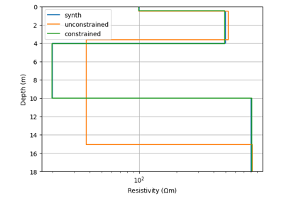
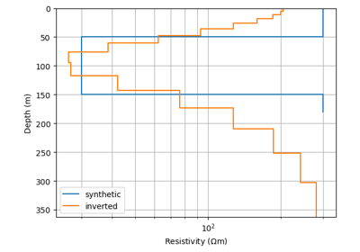
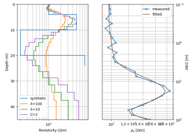
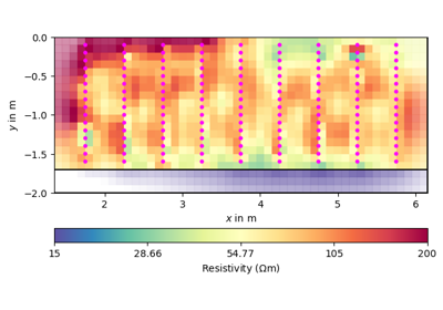
- pygimli.viewer.mpl.showStitchedModels(models, ax=None, x=None, cMin=None, cMax=None, thk=None, logScale=True, title=None, zMin=0, zMax=0, zLog=False, **kwargs)[source]#
Show several 1d block models as (stitched) section.
- Parameters:
model (iterable of iterable (np.ndarray or list of np.array)) – 1D models (consisting of thicknesses and values) to plot
ax (matplotlib axes [None - create new]) – axes object to plot in
x (iterable) – positions of individual models
cMin/cMax (float [None - autodetection from range]) – minimum and maximum colorscale range
logScale (bool [True]) – use logarithmic color scaling
zMin/zMax (float [0 - automatic]) – range for z (y axis) limits
zLog (bool) – use logarithmic z (y axis) instead of linear
topo (iterable) – vector of elevation for shifting
thk (iterable) – vector of layer thicknesses for all models
- Returns:
ax – axes object to plot in
- Return type:
matplotlib axes [None - create new]
- pygimli.viewer.mpl.showValMapPatches(vals, xVec=None, yVec=None, dx=1, dy=None, **kwargs)[source]#
Show values as patches over x and y vector.
- pygimli.viewer.mpl.showVecMatrix(xvec, yvec, vals, full=False, **kwargs)[source]#
Plot three vectors as matrix.
- Parameters:
xvec (iterable (e.g. list, np.array, pg.Vector) of identical length) – vectors defining the indices into the matrix
yvec (iterable (e.g. list, np.array, pg.Vector) of identical length) – vectors defining the indices into the matrix
vals (iterable of same length as xvec/yvec) – vector containing the values to show
full (bool [False]) – use a fully symmetric matrix containing all unique xvec+yvec otherwise A is squeezed to the individual unique xvec/yvec values
**kwargs (forwarded to plotMatrix) –
- axmpl.axis
Axis to plot, if not given a new figure is created
- cMin/cMaxfloat
Minimum/maximum color values
- logScalebool
Lgarithmic colour scale [min(A)>0]
- labelstring
Colorbar label
- Returns:
ax (matplotlib axes object) – axes object
cb (matplotlib colorbar) – colorbar object
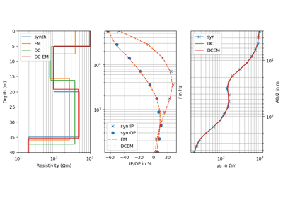
- pygimli.viewer.mpl.showfdemsounding(freq, inphase, quadrat, response=None, npl=2)[source]#
Show FDEM sounding as real(inphase) and imaginary (quadrature) fields.
- Show FDEM sounding as real(inphase) and imaginary (quadrature) fields
normalized by the (purely real) free air solution.
- pygimli.viewer.mpl.updateColorBar(cbar, gci=None, cMin=None, cMax=None, cMap=None, logScale=None, nCols=256, nLevs=5, levels=None, label=None, **kwargs)[source]#
Update colorbar values.
Update limits and label of a given colorbar.
- Parameters:
cbar (matplotlib colorbar)
gci (matplotlib graphical instance)
cMin (float)
cMax (float)
cLog (bool)
cMap (matplotlib colormap)
nCols (int [None]) – Number of colors. If not set its number of levels.
nLevs (int) – Number of color levels for the colorbar, can be different from the number of colors.
levels (iterable) – Levels for the colorbar, overwrite nLevs.
label (str) – Colorbar name.
Classes#
- class pygimli.viewer.mpl.BoreHole(fname)[source]#
Bases:
objectClass for handling (structural) borehole data for inclusion in plots.
Each row in the data file must contain a start depth [m], end depth and a classification. The values should be separated by whitespace. The first line should contain the inline position (x and z), text ID and an offset for the text (for plotting).
The format is very simple, and a sample file could look like this:
16.0 0.0 BOREHOLEID_TEXTOFFSET n 0.0 1.6 clti n 1.6 10.0 shale
- class pygimli.viewer.mpl.BoreHoles(fnames)[source]#
Bases:
objectClass to load and handle several boreholes belonging to one profile.
It makes the color coding consistent across boreholes.
- class pygimli.viewer.mpl.CellBrowser(mesh, data=None, ax=None)[source]#
Bases:
objectInteractive cell browser on current or specified ax for a given mesh.
Cell information can be displayed by mouse picking. Arrow keys up and down can be used to scroll through the cells, while ESC closes the cell information window.
- Parameters:
mesh (GIMLI::Mesh) – The plotted 2D mesh to browse through.
data (iterable) – Cell data.
ax (mpl axis instance, optional) – Axis instance where the mesh is plotted (default is current axis).
Examples
>>> import matplotlib.pyplot as plt
>>> import pygimli as pg
>>> from pygimli.viewer.mpl import drawModel
>>> from pygimli.viewer.mpl import CellBrowser
>>>
>>> mesh = pg.createGrid(range(5), range(5))
>>> fig, ax = plt.subplots()
>>> plc = drawModel(ax, mesh, mesh.cellMarkers())
>>> browser = CellBrowser(mesh)
>>> browser.connect()