Petrophysical joint inversion

Joint inversion of different geophysical techniques helps to improve both resolution and interpretability of the resulting images. Different data sets can be directly coupled, if there is a link between the target parameters. In this example, ERT and traveltime data are inverted for water saturation using petrophysical relations to resistivity and velocity. For details see section 3.3 of the pyGIMLi paper (https://cg17.pygimli.org).

import numpy as np
import pygimli as pg

from pygimli import meshtools as mt
from pygimli.physics import ert
from pygimli.physics import traveltime as tt
from pygimli.physics.petro import transFwdArchieS as ArchieTrans
from pygimli.physics.petro import transFwdWyllieS as WyllieTrans
from pygimli.frameworks import (PetroInversionManager,
                                JointPetroInversionManager)

Create synthetic model

We first set up a circular geometry with some anomalies inside.

world = mt.createCircle(boundaryMarker=-1, nSegments=64)
tri = mt.createPolygon([[-0.8, -0], [-0.5, -0.7], [0.7, 0.5]],
                        isClosed=True, area=0.0015, marker=2)
c1 = mt.createCircle(radius=0.2, pos=[-0.2, 0.5], nSegments=32,
                        area=0.0025, marker=3)
c2 = mt.createCircle(radius=0.2, pos=[0.32, -0.3], nSegments=32,
                        area=0.0025, marker=3)

poly = world + tri + c1 + c2

c = mt.createCircle(radius=0.99, nSegments=16, start=np.pi, end=np.pi*3)
for p in c.nodes():
    poly.createNode(p.pos(), -99)

poly.scale(0.2)
poly.rotate([0., 0., np.pi/3])
poly.rotate([0., 0., np.pi])

mMesh = mt.createMesh(poly, q=34.4, smooth=[1, 10])

# Create the parametric mesh that only reflects the domain geometry.
world = mt.createCircle(boundaryMarker=-1, nSegments=32, area=0.0051)
pMesh = pg.meshtools.createMesh(world, q=34.0, smooth=[1, 10])
pMesh.scale(0.2)

Mesh: Nodes: 510 Cells: 954 Boundaries: 1463

Petrophysical model

We now associate the three regions with saturation values and show the model.

saturation = pg.solver.parseArgToArray([[1, 0.6], [2, 0.9], [3, 0.3]],
                                       mMesh.cellCount(), mMesh)

satKW = dict(cMin=0.3, cMax=0.9, logScale=False, cMap="plasma_r")
ax, _ = pg.show(mMesh, saturation, **satKW,
             showMesh=True, label=r'Saturation (${\tt petro}$)')

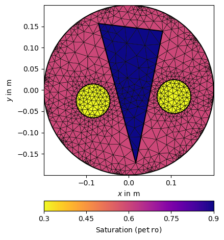
We apply the petrophysical relation to the saturation and display it with a predefined set of parameters to make all plots look the same, for both resistivity and velocity.

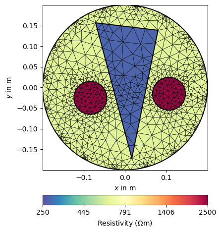
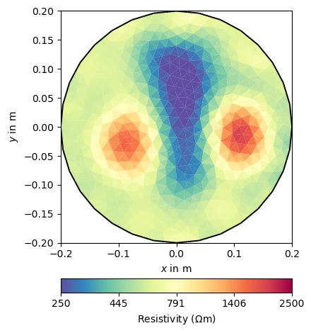
ertTrans = ArchieTrans(rFluid=20, phi=0.3)
res = ertTrans(saturation)

resKW = dict(logScale=True, cMin=250, cMax=2500,
             label=pg.unit('res'), cMap=pg.cmap('res'))

ax, _ = pg.show(mMesh, res, showMesh=True, **resKW)

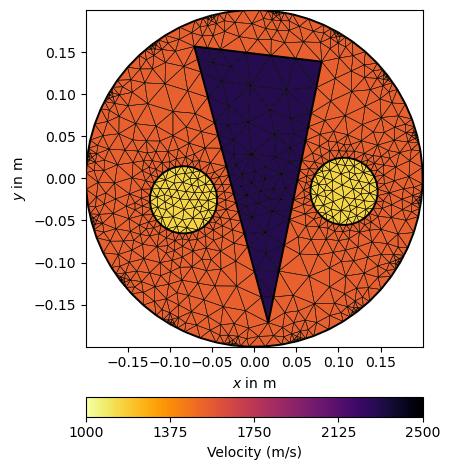
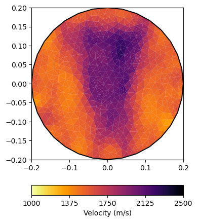
ttTrans = WyllieTrans(vm=4000, phi=0.3)
vel = 1./ttTrans(saturation)

velKW = dict(logScale=False, cMin=1000, cMax=2500,
          label=pg.unit('vel'), cMap=pg.cmap('vel'))

ax, _ = pg.show(mMesh, vel, showMesh=True, **velKW)

• 
• 

Forward simulation

To create synthetic data sets, we assume 16 equally-spaced sensors on the circumferential boundary of the mesh. For the ERT modelling we build a complete dipole-dipole array. For the ultrasonic tomography we simulate the travel time for every possible sensor pair.

sensors = mMesh.positions()[mMesh.findNodesIdxByMarker(-99)]

pg.info("Simulate ERT")
ertScheme = ert.createData(sensors, schemeName='dd', closed=1)
ertData = ert.simulate(mMesh, scheme=ertScheme, res=res, noiseLevel=0.01)

ax, _ = ert.showData(ertData, circular=True, **resKW)

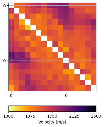
pg.info("Simulate Traveltime")
ttScheme = tt.createRAData(sensors)
ttData = tt.simulate(mMesh, scheme=ttScheme, vel=vel,
                     noiseLevel=0.01, noiseAbs=4e-6)
ax, cb = tt.showVA(ttData, **velKW)

• 
• 

/Users/fwagner/git/gimli_dev/source/pygimli/physics/ert/visualization.py:347: RuntimeWarning: invalid value encountered in cast
  ne = np.array(xe/de, dtype=int)

Conventional inversion

pg.info("ERT Inversion")
ERT = ert.ERTManager(verbose=False, sr=False)
resInv = ERT.invert(ertData, mesh=pMesh, zWeight=1, lam=20, verbose=False)
ERT.inv.echoStatus()

ax, _ = pg.show(pMesh, resInv, **resKW)

pg.info("Traveltime Inversion")
TT = tt.TravelTimeManager(verbose=False)
velInv = TT.invert(ttData, mesh=pMesh, lam=100, useGradient=0, zWeight=1.0)
TT.inv.echoStatus()

ax, _ = pg.show(pMesh, velInv, **velKW)

• 
• 

Petrophysical inversion (individually)

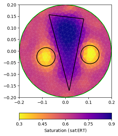
pg.info("ERT Petrogeophysical Inversion")
ERTPetro = PetroInversionManager(petro=ertTrans, mgr=ERT)
satERT = ERTPetro.invert(ertData, mesh=pMesh, limits=[0., 1.], lam=10,
                         verbose=False)
ERTPetro.inv.echoStatus()

ax, _ = pg.show(pMesh, satERT, **satKW, label=r'Saturation (${\tt satERT}$)')
pg.viewer.mpl.drawPLC(ax, poly, fillRegion=False)

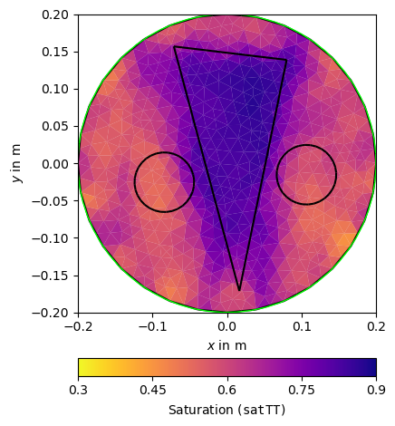
pg.info("TT Petrogeophysical Inversion")
TTPetro = PetroInversionManager(petro=ttTrans, mgr=TT)
satTT = TTPetro.invert(ttData, mesh=pMesh, limits=[0., 1.], lam=5)
TTPetro.inv.echoStatus()

ax, _ = pg.show(pMesh, satTT, **satKW, label=r'Saturation (${\tt satTT}$)')
pg.viewer.mpl.drawPLC(ax, poly, fillRegion=False)

• 
• 

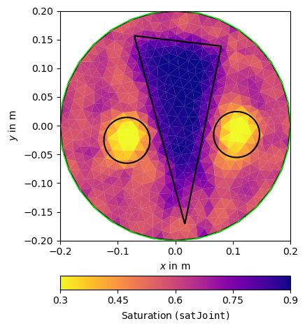
Petrophysical joint inversion

pg.info("Petrophysical Joint-Inversion TT-ERT")
JointPetro = JointPetroInversionManager(petros=[ertTrans, ttTrans],
                                        mgrs=[ERT, TT])
satJoint = JointPetro.invert([ertData, ttData], mesh=pMesh,
                             limits=[0., 1.], lam=5, verbose=False)
JointPetro.inv.echoStatus()

ax, _ = pg.show(pMesh, satJoint, **satKW, label=r'Saturation (${\tt satJoint}$)')
pg.viewer.mpl.drawPLC(ax, poly, fillRegion=False)