3D surface ERT inversion

Inversion of 3D surface ERT field data (the gallery) The data was measured by T. Günther and F. Donner in 2000 with the ERT instrument of the TU Bergakademie Freiberg and used for the PhD thesis of Günther (2004).

We import the pygimli library and toolboxes for mesh, plot and ERT.

import pygimli as pg
import pygimli.meshtools as mt
from pygimli.physics import ert
from pygimli.viewer import pv

We load the data file from the example repository. It represents a surface ERT array in a 14x9 electrode grid with a spacing of 2.5m (Günther, 2004). Data are measured using the dipole-dipole array in both x and y direction.

data = pg.getExampleData("ert/gallery3d.dat")
data["k"] = ert.geometricFactors(data, dim=3)
print(data)

Data: Sensors: 126 data: 753, nonzero entries: ['a', 'b', 'k', 'm', 'n', 'rhoa', 'valid']

For generating the mesh, we first create a piecewise-linear complex, i.e. the boxes for inversion region and background and mesh it then.

plc = mt.createParaMeshPLC3D(data, paraDepth=12, paraMaxCellSize=3,
                             surfaceMeshQuality=34)
mesh = mt.createMesh(plc, quality=1.3)
print(mesh)

Mesh: Nodes: 2689 Cells: 14227 Boundaries: 29159

We estimate an error using 2% relative error and an absolute error of 100uV at an assumed current of 100mA which is almost zero.

data["err"] = ert.estimateError(data, relativeError=0.02)
mgr = ert.ERTManager(data)
mgr.invert(mesh=mesh, verbose=True)

fop: <pygimli.physics.ert.ertModelling.ERTModelling object at 0x3276898f0>
Data transformation: Logarithmic LU transform, lower bound 0.0, upper bound 0.0
Model transformation: Logarithmic transform
min/max (data): 119/488
min/max (error): 2%/2%
min/max (start model): 257/257
--------------------------------------------------------------------------------
inv.iter 0 ... chi² =  217.79
--------------------------------------------------------------------------------
inv.iter 1 ... chi² =   16.52 (dPhi = 90.92%) lam: 20.0
--------------------------------------------------------------------------------
inv.iter 2 ... chi² =    4.11 (dPhi = 58.82%) lam: 20.0
--------------------------------------------------------------------------------
inv.iter 3 ... chi² =    3.09 (dPhi = 11.94%) lam: 20.0
--------------------------------------------------------------------------------
inv.iter 4 ... chi² =    2.96 (dPhi = 1.27%) lam: 20.0
################################################################################
#                Abort criterion reached: dPhi = 1.27 (< 2.0%)                 #
################################################################################

6800 [457.26305089798797,...,398.70419140360895]

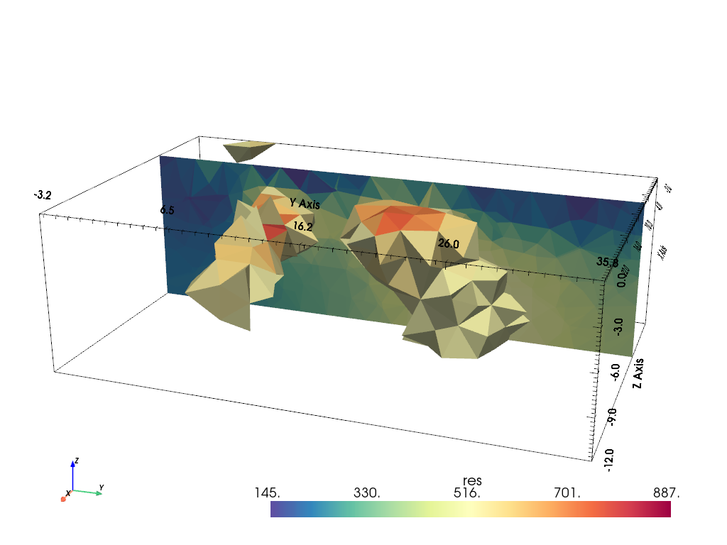
We visualize the result by a resistivity threshold and a slice using pyVista

pd = mgr.paraDomain
pd["res"] = mgr.model
pl, _ = pg.show(pd, label="res", style="surface", cMap="Spectral_r", hold=True,
                filter={"threshold": dict(value=500, scalars="res")})
pv.drawMesh(pl, pd, label="res", style="surface", cMap="Spectral_r",
            filter={"slice": dict(normal=[-1, 0, 0], origin=[5, 15, -2])})
pl.camera_position = "yz"
pl.camera.azimuth = 20
pl.camera.elevation = 20
pl.camera.zoom(1.2)
_ = pl.show()

References

Günther, T. (2004): Inversion Methods and Resolution Analysis for the 2D/3D Reconstruction of Resistivity Structures from DC Measurements. PhD thesis, University of Mining and Technology, Freiberg, available on http://nbn-resolving.de/urn:nbn:de:swb:105-4152277.