Note
Go to the end to download the full example code.
Incorporating additional constraints as equations#
Sometimes we have additional information on the model that can be expressed in form of an equation. Let us consider a simple vertical electrical sounding (VES) that is inverted for a four-layer case with unknown layer thicknesses.
Assume we know the depth of the layer boundary, e.g. from a borehole, in this case between the third and fourth layer be \(z_2\). So we can formulate this by an equation \(d_1+d_2+d_3=z_2\). This equation is added to the inverse problem in the style of Lagrangian, i.e., by an additional regularization term.
We use the LSQR inversion framework as used by Wagner et al. (2019) to constrain the sum of water, ice, air and rock fraction to be 1.
import numpy as np
import matplotlib.pyplot as plt
import pygimli as pg
from pygimli.frameworks.lsqrinversion import LSQRInversion
from pygimli.physics.ves import VESModelling
from pygimli.viewer.mpl import drawModel1D
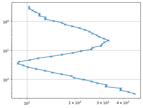
We set up a synthetic model of four layers and show the sounding curve
nlay = 4  # number of layers
lam = 200.  # (initial) regularization parameter
errPerc = 3.  # relative error of 3 percent
ab2 = np.logspace(-0.5, 2.5, 50)  # AB/2 distance (current electrodes)
mn2 = ab2 / 3.  # MN/2 distance (potential electrodes)
f = VESModelling(ab2=ab2, mn2=mn2, nLayers=nlay)
synres = [100., 500., 20., 800.]  # synthetic resistivity
synthk = [0.5, 3.5, 6.]  # synthetic thickness (nlay-th layer is infinite)
rhoa = f(synthk+synres)
rhoa = rhoa * (pg.randn(len(rhoa)) * errPerc / 100. + 1.)
fig, ax = plt.subplots()
ax.loglog(rhoa, ab2, "x-")
ax.invert_yaxis()
ax.grid(True)
Next, we set up an inversion instance with log transformation on data and model side and run the inversion.
inv = LSQRInversion(fop=f, verbose=True)
inv.dataTrans = 'log'
inv.modelTrans = 'log'
startModel = [7.0] * (nlay-1) + [pg.median(rhoa)] * nlay
inv.inv.setMarquardtScheme()
model1 = inv.run(rhoa, errPerc/100, lam=lam, startModel=startModel)
fop: <pygimli.physics.ves.vesModelling.VESModelling object at 0x173595670>
Data transformation: Logarithmic transform
Model transformation (cumulative):
         0 Logarithmic LU transform, lower bound 0.0, upper bound 0.0
         1 Logarithmic LU transform, lower bound 0.0, upper bound 0.0
min/max (data): 87.26/473
min/max (error): 3%/3%
min/max (start model): 7/193
--------------------------------------------------------------------------------
inv.iter 0 ... chi² =  234.24
--------------------------------------------------------------------------------
inv.iter 1 ... chi² =  196.77 (dPhi = 16.00%) lam: 200.0
--------------------------------------------------------------------------------
inv.iter 2 ... chi² =  185.59 (dPhi = 5.68%) lam: 200.0
--------------------------------------------------------------------------------
inv.iter 3 ... chi² =  167.14 (dPhi = 9.94%) lam: 200.0
--------------------------------------------------------------------------------
inv.iter 4 ... chi² =  151.58 (dPhi = 9.31%) lam: 200.0
--------------------------------------------------------------------------------
inv.iter 5 ... chi² =  121.45 (dPhi = 19.88%) lam: 200.0
--------------------------------------------------------------------------------
inv.iter 6 ... chi² =   85.24 (dPhi = 29.82%) lam: 200.0
--------------------------------------------------------------------------------
inv.iter 7 ... chi² =   64.51 (dPhi = 24.31%) lam: 200.0
--------------------------------------------------------------------------------
inv.iter 8 ... chi² =   22.57 (dPhi = 65.01%) lam: 200.0
--------------------------------------------------------------------------------
inv.iter 9 ... chi² =    2.87 (dPhi = 87.30%) lam: 200.0
--------------------------------------------------------------------------------
inv.iter 10 ... chi² =    1.01 (dPhi = 64.84%) lam: 200.0
--------------------------------------------------------------------------------
inv.iter 11 ... chi² =    0.89 (dPhi = 11.94%) lam: 200.0


################################################################################
#                  Abort criterion reached: chi² <= 1 (0.89)                   #
################################################################################
To formulate the constraints, we need to set up a matrix for the left side and a vector for the right side of the equation. The layer thicknesses are the first values in the model vector, and setting 1 implements d1+d2+d3:
d1 d2 d3 r1 r2 r3 r4
G = [1 1 1 0 0 0 0] c = [z2] The constraints G * m = c are set by setParameterConstraints with a Lagrangian parameter that determines how well the equation needs to be fit.
G = pg.Matrix(rows=1, cols=len(startModel))
for i in range(3):
    G.setVal(0, i, 1)

c = pg.Vector(1, pg.sum(synthk))
inv.setParameterConstraints(G, c, 100)
model2 = inv.run(rhoa, errPerc/100, lam=lam, startModel=startModel)
fop: <pygimli.physics.ves.vesModelling.VESModelling object at 0x173595670>
Data transformation: Logarithmic transform
Model transformation (cumulative):
         0 Logarithmic LU transform, lower bound 0.0, upper bound 0.0
         1 Logarithmic LU transform, lower bound 0.0, upper bound 0.0
min/max (data): 87.26/473
min/max (error): 3%/3%
min/max (start model): 7/193
--------------------------------------------------------------------------------
inv.iter 0 ... chi² =  234.24
--------------------------------------------------------------------------------
inv.iter 1 ... chi² =  155.51 (dPhi = 33.61%) lam: 200.0
--------------------------------------------------------------------------------
inv.iter 2 ... chi² =  133.71 (dPhi = 14.02%) lam: 200.0
--------------------------------------------------------------------------------
inv.iter 3 ... chi² =  120.16 (dPhi = 10.13%) lam: 200.0
--------------------------------------------------------------------------------
inv.iter 4 ... chi² =  104.62 (dPhi = 12.94%) lam: 200.0
--------------------------------------------------------------------------------
inv.iter 5 ... chi² =   59.02 (dPhi = 43.58%) lam: 200.0
--------------------------------------------------------------------------------
inv.iter 6 ... chi² =   36.79 (dPhi = 37.66%) lam: 200.0
--------------------------------------------------------------------------------
inv.iter 7 ... chi² =    8.69 (dPhi = 76.38%) lam: 200.0
--------------------------------------------------------------------------------
inv.iter 8 ... chi² =    1.15 (dPhi = 86.82%) lam: 200.0
--------------------------------------------------------------------------------
inv.iter 9 ... chi² =    0.88 (dPhi = 22.89%) lam: 200.0


################################################################################
#                  Abort criterion reached: chi² <= 1 (0.88)                   #
################################################################################
All three models are plotted together and are equivalently fitting the data. Due to the additional constraints, the model is much closer to the synthetic.
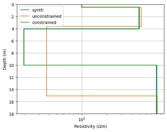
<matplotlib.legend.Legend object at 0x329a63980>
References#
- Wagner, F.M., Mollaret, C., Günther, T., Kemna, A., Hauck, A. (2019):
Quantitative imaging of water, ice, and air in permafrost systems through petrophysical joint inversion of seismic refraction and electrical resistivity data. Geophys. J. Int. 219, 1866-1875. doi:10.1093/gji/ggz402.