Note
Go to the end to download the full example code.
Incorporating prior data into ERT inversion#
Prior data can often help to overcome ambiguity in the inversion process. Here we demonstrate the use of direct push (DP) data in an ERT inversion of data collected at the surface.
import matplotlib.pyplot as plt
import numpy as np
import pygimli as pg
from pygimli.physics import ert
from pygimli.frameworks import PriorModelling, JointModelling
from pygimli.viewer.mpl import draw1DColumn
The prior data#
This field data is from a site with layered sands and clays over a resistive bedrock. We load it from the example repository.
As a position of x=155m (center of the profile) we have a borehole/direct push with known in-situ-data. We load the three-column file using numpy.
x, z, r = pg.getExampleData("ert/bedrock.txt").T
fig, ax = plt.subplots()
ax.semilogx(r, z, "*-")
ax.set_xlabel(r"$\rho$ ($\Omega$m)")
ax.set_ylabel("depth (m)")
ax.grid(True)
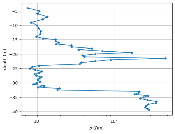
We mainly see four layers: 1. a conductive (clayey) overburden of about 17m thickness, 2. a medium resistivity interbedding of silt and sand, about 7m thick 3. again clay with 8m thickness 4. the resistive bedrock with a few hundred :math:`Omega`m
The ERT data#
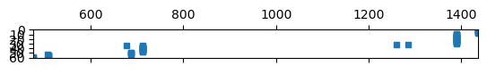
We load the ERT data from the example repository and plot the pseudosection.
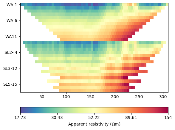
Data: Sensors: 64 data: 1223, nonzero entries: ['a', 'b', 'err', 'm', 'n', 'rhoa', 'valid']
The apparent resistivities show increasing values with larger spacings with no observable noise. We first compute geometric factors and estimate an error model using rather low values for both error parts.
data.estimateError(relativeError=0.025, absoluteUError=100e-6)
# data["k"] = ert.geometricFactors(data)
# data["err"] = ert.estimateError(data, relativeError=0.025, absoluteUError=100e-6)
We create an ERT manager and invert the data, already using a rather low value for the vertical smoothness to account for the layered model.
mgr = ert.ERTManager(data, verbose=True)
mgr.invert(paraDepth=70, quality=34.2, paraMaxCellSize=1000, zWeight=0.15, lam=30)
fop: <pygimli.physics.ert.ertModelling.ERTModelling object at 0x323cb6890>
Data transformation: Logarithmic LU transform, lower bound 0.0, upper bound 0.0
Model transformation (cumulative):
         0 Logarithmic LU transform, lower bound 0.0, upper bound 0.0
min/max (data): 17.73/154
min/max (error): 2.54%/4.38%
min/max (start model): 48.34/48.34
--------------------------------------------------------------------------------
inv.iter 0 ... chi² =  241.67
--------------------------------------------------------------------------------
inv.iter 1 ... chi² =    4.47 (dPhi = 98.00%) lam: 30.0
--------------------------------------------------------------------------------
inv.iter 2 ... chi² =    4.24 (dPhi = 5.10%) lam: 30.0
--------------------------------------------------------------------------------
inv.iter 3 ... chi² =    4.03 (dPhi = 4.86%) lam: 30.0
--------------------------------------------------------------------------------
inv.iter 4 ... chi² =    3.46 (dPhi = 14.18%) lam: 30.0
--------------------------------------------------------------------------------
inv.iter 5 ... chi² =    3.20 (dPhi = 7.85%) lam: 30.0
--------------------------------------------------------------------------------
inv.iter 6 ... chi² =    2.99 (dPhi = 6.58%) lam: 30.0
--------------------------------------------------------------------------------
inv.iter 7 ... chi² =    2.70 (dPhi = 9.71%) lam: 30.0
--------------------------------------------------------------------------------
inv.iter 8 ... chi² =    1.36 (dPhi = 46.13%) lam: 30.0
--------------------------------------------------------------------------------
inv.iter 9 ... chi² =    0.20 (dPhi = 74.44%) lam: 30.0


################################################################################
#                  Abort criterion reached: chi² <= 1 (0.20)                   #
################################################################################

1593 [32.563898976671815,...,410.54608527105324]
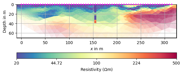
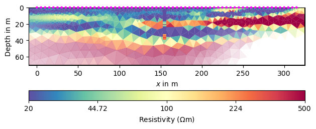
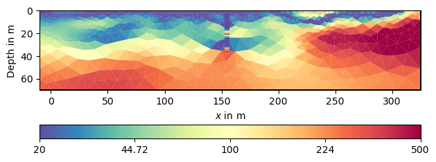
For reasons of comparability, we define a unique colormap and store all options in a dictionary to be used in subsequent show commands.
We plot the result with these and plot the DP points onto the mesh.
kw = dict(cMin=20, cMax=500, logScale=True, cMap="Spectral_r",
          xlabel="x (m)", ylabel="y (m)")
ax, cb = mgr.showResult(**kw)
zz = np.abs(z)
iz = np.argsort(z)
dz = np.diff(zz[iz])
thk = np.hstack([dz, dz[-1]])
ztop = -zz[iz[0]]-dz[0]/2
colkw = dict(x=x[0], val=r[iz], thk=thk, width=4, ztopo=ztop)
draw1DColumn(ax, **colkw, **kw)
ax.grid(True)
We want to extract the resistivity from the mesh at the positions where
the prior data are available. To this end, we create a list of positions
(pg.Pos class) and use a forward operator that picks the values from a
model vector according to the cell where the position is in. See the
regularization tutorial for details about that.
We can now use it to retrieve the model values, store it and plot it along with the measured values.
fig, ax = plt.subplots()
ax.semilogx(r, z, label="borehole")
resSmooth = fopDP(mgr.model)
ax.semilogx(resSmooth, z, label="ERT")
ax.set_xlabel(r"$\rho$ ($\Omega$m)")
ax.set_ylabel("depth (m)")
ax.grid(True)
ax.legend()
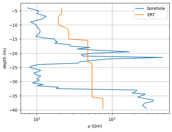
<matplotlib.legend.Legend object at 0x3299d98b0>
As alternative to smoothness, we can use a geostatistic model. The vertical range can be well estimated from the DP data using a variogram analysis, we guess 8m. For the horizontal one, we can only guess a ten times higher value.
fop: <pygimli.physics.ert.ertModelling.ERTModelling object at 0x323cb6890>
Data transformation: Logarithmic LU transform, lower bound 0.0, upper bound 0.0
Model transformation (cumulative):
         0 Logarithmic LU transform, lower bound 0.0, upper bound 0.0
min/max (data): 17.73/154
min/max (error): 2.54%/4.38%
min/max (start model): 48.34/48.34
--------------------------------------------------------------------------------
inv.iter 0 ... chi² =  241.67
--------------------------------------------------------------------------------
inv.iter 1 ... chi² =   40.68 (dPhi = 83.05%) lam: 20.0
--------------------------------------------------------------------------------
inv.iter 2 ... chi² =    6.80 (dPhi = 83.10%) lam: 20.0
--------------------------------------------------------------------------------
inv.iter 3 ... chi² =    0.55 (dPhi = 90.13%) lam: 20.0


################################################################################
#                  Abort criterion reached: chi² <= 1 (0.55)                   #
################################################################################
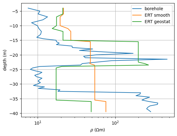
Let’s compare the three resistivity soundings with the ground truth.
fig, ax = plt.subplots()
ax.semilogx(r, z, label="borehole")
ax.semilogx(resSmooth, z, label="ERT smooth")
# ax.semilogx(res2, z, label="ERT aniso")
ax.semilogx(resGeo, z, label="ERT geostat")
ax.set_xlabel(r"$\rho$ ($\Omega$m)")
ax.set_ylabel("depth (m)")
ax.grid()
ax.legend()
<matplotlib.legend.Legend object at 0x323e507a0>
The anisotropic regularization starts to see the good conductor, but only the geostatistical regularization operator is able to retrieve values that are close to the direct push. Both show the conductor too deep.
One alternative could be to use the interfaces as structural constraints in the neighborhood of the borehole. See ERT with structural constraints example
As the DP data is not only good for comparison, we want to use its values as data in inversion. This is easily accomplished by taking the mapping operator that we already use for interpolation as a forward operator.
We set up an inversion with this mesh, logarithmic transformations and invert the model.
fop: <pygimli.frameworks.modelling.PriorModelling object at 0x3552cbc40>
Data transformation: Logarithmic transform
Model transformation (cumulative):
         0 Logarithmic LU transform, lower bound 0.0, upper bound 0.0
min/max (data): 7.52/469
min/max (error): 20%/20%
min/max (start model): 17.84/17.84
--------------------------------------------------------------------------------
inv.iter 0 ... chi² =   55.40
--------------------------------------------------------------------------------
inv.iter 1 ... chi² =   21.59 (dPhi = 59.93%) lam: 20.0
--------------------------------------------------------------------------------
inv.iter 2 ... chi² =   21.59 (dPhi = 0.44%) lam: 20.0
--------------------------------------------------------------------------------
inv.iter 3 ... chi² =   21.59 (dPhi = 0.19%) lam: 20.0
################################################################################
#                Abort criterion reached: dPhi = 0.19 (< 2.0%)                 #
################################################################################

<matplotlib.collections.PatchCollection object at 0x323c856a0>
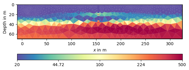
Apparently, the geostatistical operator can be used to extrapolate values with given assumptions.
Joint inversion of ERT and DP data#
We now use the framework JointModelling to combine the ERT and the
DP forward operators. So we set up a new ERT modelling operator and join
it with fopDP.
# fopERT = ert.ERTModelling()
# fopERT.setMesh(mesh)
# fopERT.setData(data) # not necessary as done by JointModelling
# fopJoint = JointModelling([fopERT, fopDP])
fopJoint = JointModelling([mgr.fop, fopDP])
# fopJoint.setMesh(para)
fopJoint.setData([data, pg.Vector(r)])  # needs to have .size() attribute!
We first test the joint forward operator. We create a modelling vector of constant resistivity and distribute the model response into the two parts that can be looked at individually.
[100.0, 100.0, 100.0, 100.0, 100.0, 100.0, 100.0, 100.0, 100.0, 100.0, 100.0, 100.0, 100.0, 100.0, 100.0, 100.0, 100.0, 100.0, 100.0, 100.0, 100.0, 100.0, 100.0, 100.0, 100.0, 100.0, 100.0, 100.0, 100.0, 100.0, 100.0, 100.0, 100.0, 100.0, 100.0, 100.0, 100.0, 100.0, 100.0, 100.0, 100.0, 100.0, 100.0, 100.0, 100.0, 100.0, 100.0, 100.0, 100.0, 100.0, 100.0, 100.0, 100.0, 100.0, 100.0, 100.0, 100.0, 100.0, 100.0, 100.0, 100.0, 100.0]
The jacobian can be created and looked up by
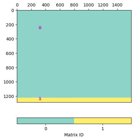
<class 'pygimli.core.libs._pygimli_.RBlockMatrix'>
RMatrix: 1223 x 1593
For the joint inversion, concatenate the data and error vectors, create a new inversion instance, set logarithmic transformations and run the inversion.
dataVec = np.concatenate((data["rhoa"], r))
errorVec = np.concatenate((data["err"], np.ones_like(r)*0.2))
inv = pg.Inversion(fop=fopJoint, verbose=True)
transLog = pg.trans.TransLog()
inv.modelTrans = transLog
inv.dataTrans = transLog
inv.run(dataVec, errorVec, startModel=model)
ax, cb = pg.show(para, inv.model, **kw)
draw1DColumn(ax, **colkw, **kw)
fop: <pygimli.frameworks.modelling.JointModelling object at 0x32b4590d0>
Data transformation: Logarithmic transform
Model transformation (cumulative):
         0 Logarithmic LU transform, lower bound 0.0, upper bound 0.0
min/max (data): 7.52/469
min/max (error): 2.54%/20%
min/max (start model): 100/100
--------------------------------------------------------------------------------
inv.iter 0 ... chi² =  788.14
--------------------------------------------------------------------------------
inv.iter 1 ... chi² =    5.29 (dPhi = 99.30%) lam: 20.0
--------------------------------------------------------------------------------
inv.iter 2 ... chi² =    4.39 (dPhi = 16.76%) lam: 20.0
--------------------------------------------------------------------------------
inv.iter 3 ... chi² =    3.53 (dPhi = 19.37%) lam: 20.0
--------------------------------------------------------------------------------
inv.iter 4 ... chi² =    1.44 (dPhi = 56.54%) lam: 20.0
--------------------------------------------------------------------------------
inv.iter 5 ... chi² =    1.22 (dPhi = 13.88%) lam: 20.0
--------------------------------------------------------------------------------
inv.iter 6 ... chi² =    1.19 (dPhi = 1.85%) lam: 20.0
################################################################################
#                Abort criterion reached: dPhi = 1.85 (< 2.0%)                 #
################################################################################

<matplotlib.collections.PatchCollection object at 0x32ab4edb0>
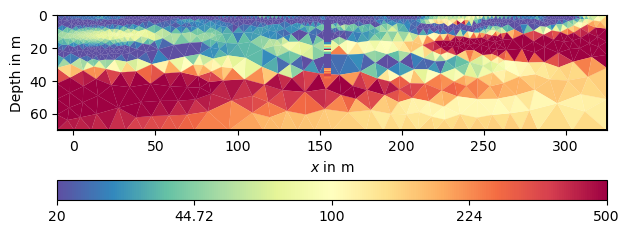
We have a local improvement of the model in the neighborhood of the borehole. Now we want to use geostatistics to get them further into the model.
fop: <pygimli.frameworks.modelling.JointModelling object at 0x32b4590d0>
Data transformation: Logarithmic transform
Model transformation (cumulative):
         0 Logarithmic LU transform, lower bound 0.0, upper bound 0.0
min/max (data): 7.52/469
min/max (error): 2.54%/20%
min/max (start model): 100/100
--------------------------------------------------------------------------------
inv.iter 0 ... chi² =  788.14
--------------------------------------------------------------------------------
inv.iter 1 ... chi² =   14.52 (dPhi = 98.13%) lam: 20.0
--------------------------------------------------------------------------------
inv.iter 2 ... chi² =    5.49 (dPhi = 61.83%) lam: 20.0
--------------------------------------------------------------------------------
inv.iter 3 ... chi² =    2.47 (dPhi = 53.33%) lam: 20.0
--------------------------------------------------------------------------------
inv.iter 4 ... chi² =    2.37 (dPhi = 4.08%) lam: 20.0
--------------------------------------------------------------------------------
inv.iter 5 ... chi² =    1.82 (dPhi = 22.03%) lam: 20.0
--------------------------------------------------------------------------------
inv.iter 6 ... chi² =    1.22 (dPhi = 29.97%) lam: 20.0
--------------------------------------------------------------------------------
inv.iter 7 ... chi² =    1.22 (dPhi = 0.00%) lam: 20.0
################################################################################
#                 Abort criterion reached: dPhi = 0.0 (< 2.0%)                 #
################################################################################

<matplotlib.collections.PatchCollection object at 0x329d3e270>
This model much better resembles the subsurface from all data and our expectations to it.
We split the model response in the ERT part and the DP part. The first is shown as misfit.
respERT = inv.response[:data.size()]
misfit = - respERT / data["rhoa"] * 100 + 100
# ax, cb = ert.show(data, misfit, cMap="bwr", cMin=-5, cMax=5)
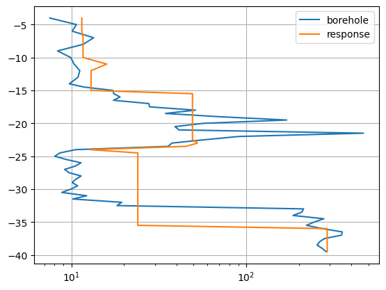
The second is shown as depth profile.
respDP = inv.response[data.size():]
fig, ax = plt.subplots()
ax.semilogx(r, z, label="borehole")
# resMesh = pg.interpolate(srcMesh=para, inVec=inv.model, destPos=posVec)
# ax.semilogx(resMesh, z, label="ERT+DP")
ax.semilogx(respDP, z, label="response")
ax.grid(True)
ax.legend()
<matplotlib.legend.Legend object at 0x355700230>
The model response can much better resemble the given data compared to pure interpolation. However, at shallow depth there is some inconsistency between the ERT data and the borehole data.
Note
Take-away messages
(ERT) data inversion is highly ambiguous, particularly for hidden layers
prior data can help to improve regularization
point data improve images, but only locally with smoothness constraints
geostatistical regularization can extrapolate point data
incorporation of prior data with geostatistic regularization is best
Total running time of the script: (1 minutes 1.627 seconds)