ERT field data with topography

Simple example of data measured over a slagdump demonstrating:

• 2D inversion with topography

• geometric factor generation

• topography effect

The data is the profile 11 already shown by Günther et al. (2006, Fig. 11).

import matplotlib.pyplot as plt
import pygimli as pg
from pygimli.physics import ert

Get some example data with, typically by a call like data = ert.load(“filename.dat”) that supports various file formats

data = pg.getExampleData('ert/slagdump.ohm', verbose=True)
print(data)

Data: Sensors: 38 data: 222, nonzero entries: ['a', 'b', 'm', 'n', 'r', 'valid']

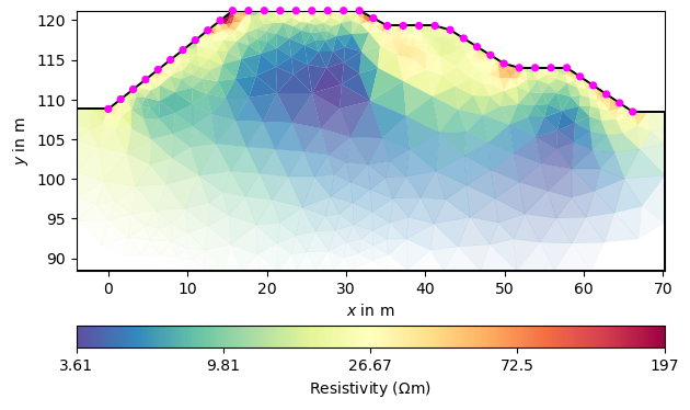
Let us first have a look at the topography contained in the data

plt.plot(pg.x(data), pg.z(data), 'x-')

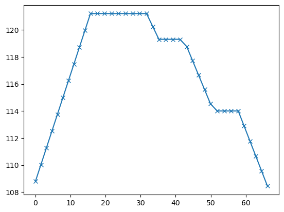
[<matplotlib.lines.Line2D object at 0x172c37380>]

The data file does not contain geometric factors (token field ‘k’), so we create them based on the given topography.

k0 = ert.createGeometricFactors(data)  # the analytical one
data['k'] = ert.createGeometricFactors(data, numerical=True)

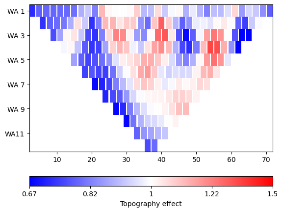
It might be interesting to see the topography effect, i.e the ratio between the numerically computed geometry factor and the analytical formula after Rücker et al. (2006). We display it using a colormap with neutral white.

_ = ert.showData(data, vals=k0/ data['k'], label='Topography effect',
                 cMin=2/3, cMax=3/2, logScale=True, cMap="bwr")

We can now compute the apparent resistivity and display it, once with the wrong analytical formula and once with the numerical values in data[‘k’]

data['rhoa'] = data['r'] * data['k']
kw = dict(cMin=6, cMax=33)
fig, ax = plt.subplots(ncols=2)
data.show(data['r']*k0, ax=ax[0], **kw);
data.show(ax=ax[1], **kw)
ax[0].set_title('Uncorrected')
ax[1].set_title('Corrected');

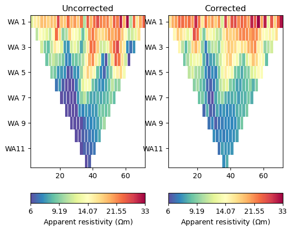
Text(0.5, 1.0, 'Corrected')

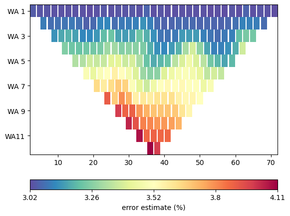
The data container does not necessarily contain data errors data errors (token field ‘err’), requiring us to enter data errors. We can let the manager guess some defaults for us automaticly or set them manually

data.estimateError(relativeError=0.03, absoluteUError=5e-5)
# which internally calls
# data['err'] = ert.estimateError(data, ...)  # can also set manually
_ = data.show(data['err']*100, label='error estimate (%)')

We initialize the ERTManager for further steps and eventually inversion.

mgr = ert.ERTManager(data)

Now the data have all necessary fields (‘rhoa’, ‘err’ and ‘k’) so we can run the inversion. The inversion mesh will be created with some optional values for the parametric mesh generation.

mod = mgr.invert(data, lam=10, verbose=True,
                 paraDX=0.3, paraMaxCellSize=10, paraDepth=20, quality=33.6)
ax, cb = mgr.showResult()

fop: <pygimli.physics.ert.ertModelling.ERTModelling object at 0x323504540>
Data transformation: Logarithmic LU transform, lower bound 0.0, upper bound 0.0
Model transformation: Logarithmic transform
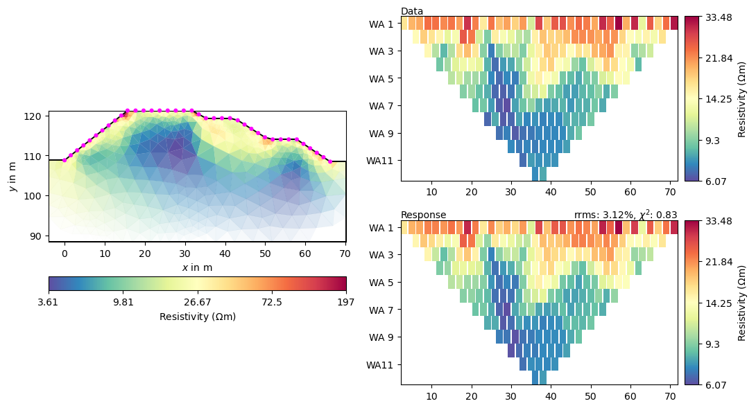
min/max (data): 6.07/33.48
min/max (error): 3.02%/4.11%
min/max (start model): 10.65/10.65
--------------------------------------------------------------------------------
inv.iter 0 ... chi² =  198.11
--------------------------------------------------------------------------------
inv.iter 1 ... chi² =   16.04 (dPhi = 90.58%) lam: 10.0
--------------------------------------------------------------------------------
inv.iter 2 ... chi² =    1.27 (dPhi = 81.89%) lam: 10.0
--------------------------------------------------------------------------------
inv.iter 3 ... chi² =    0.83 (dPhi = 10.20%) lam: 10.0


################################################################################
#                  Abort criterion reached: chi² <= 1 (0.83)                   #
################################################################################

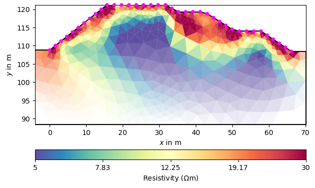
We can view the resulting model in the usual way.

_ = mgr.showResultAndFit()
# np.testing.assert_approx_equal(ert.inv.chi2(), 1.10883, significant=3)

Or just plot the model only using your own options.

ax, cb = mgr.showResult(mod, cMin=5, cMax=30, cMap="Spectral_r", logScale=True)