Refraction in 3D

This example shows refracted ray paths in a three-dimensional vertical gradient medium.

Note

This is a placeholder/proof-of-concept. The code should be refactored partly to tt.showRayPaths()

import numpy as np
import pygimli as pg
import pygimli.meshtools as mt
from pygimli.physics import traveltime as tt
from pygimli.viewer.pv import drawSensors
import pyvista

Build mesh.

depth = 15
width = 30
plc = mt.createCube(size=[width, width, depth], pos=[0, 0, -depth/2], area=5)

n_sensors = 8
sensors = np.zeros((n_sensors, 3))
sensors[0, 0] = 15
sensors[0, 1] = -10
sensors[1:, 0] = -15
sensors[1:, 1] = np.linspace(-15, 15, n_sensors - 1)

for pos in sensors:
    plc.createNode(pos)
mesh = mt.createMesh(plc)
mesh.createSecondaryNodes(1)

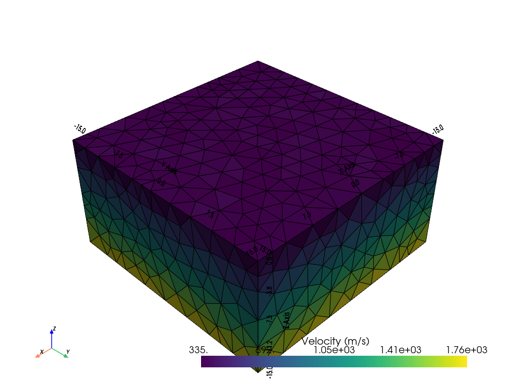
Create vertical gradient model.

vel = 300 + -pg.z(mesh.cellCenters()) * 100
pg.show(mesh, vel, label=pg.utils.unit("vel"), showMesh=True)

(<pyvista.plotting.plotter.Plotter object at 0x141af5fa0>, None)

Set-up data container.

data = tt.createRAData(sensors)
data.markInvalid(data("s") > 1)
data.set("t", np.zeros(data.size()))
data.removeInvalid()

Do raytracing.

# fop = pg.core.TravelTimeDijkstraModelling(mesh, data)
fop = tt.TravelTimeModelling()
fop.setData(data)
fop.setMesh(mesh)
print(fop.mesh())

# This is to show single raypaths.
graph = fop.createGraph(1 / vel)
dij = tt.Dijkstra(graph)
dij.setStartNode(mesh.findNearestNode([15, -10, 0]))

rays = []
for receiver in sensors[1:]:
    ni = dij.shortestPathTo(mesh.findNearestNode(receiver))
    pos = mesh.positions(withSecNodes=True)[ni]
    segs = np.zeros((len(pos), 3))
    segs[:,0] = pg.x(pos)
    segs[:,1] = pg.y(pos)
    segs[:,2] = pg.z(pos)
    rays.append(segs)

Mesh: Nodes: 1115 Cells: 4988 Boundaries: 10542 secNodes: 17210

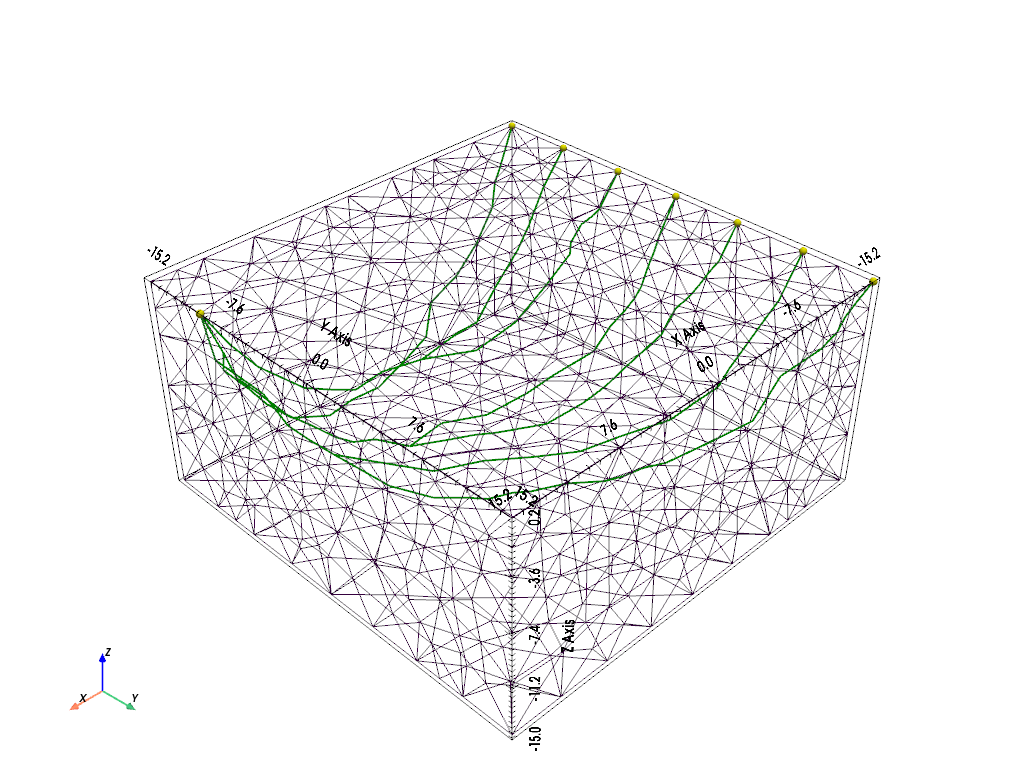
Plot final ray paths.

pl, _ = pg.show(mesh, style='wireframe', line_width=0.1,
                        hold=True)
drawSensors(pl, sensors, diam=0.5, color='yellow')

for ray in rays:
    for i in range(len(ray) - 1):
        start = tuple(ray[i])
        stop = tuple(ray[i + 1])
        line = pyvista.Line(start, stop)
        pl.add_mesh(line, color='green', line_width=2)

pl.show()