2D Refraction modelling and inversion

This example shows how to use the TravelTime manager to generate the response of a three-layered sloping model and to invert the synthetic noisified data.

import numpy as np
import pygimli as pg
import pygimli.meshtools as mt
import pygimli.physics.traveltime as tt

Model setup

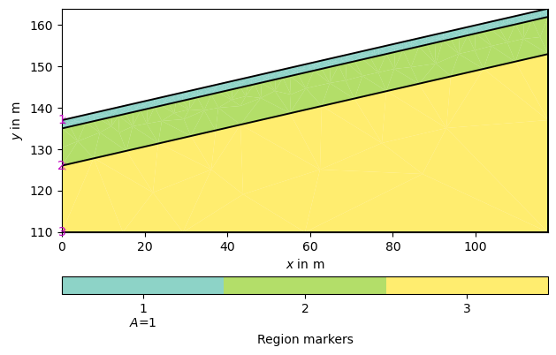
We start by creating a three-layered slope (The model is taken from the BSc thesis of Constanze Reinken conducted at the University of Bonn).

layer1 = mt.createPolygon([[0.0, 137], [117.5, 164], [117.5, 162], [0.0, 135]],
                          isClosed=True, marker=1, area=1)
layer2 = mt.createPolygon([[0.0, 126], [0.0, 135], [117.5, 162], [117.5, 153]],
                          isClosed=True, marker=2)
layer3 = mt.createPolygon([[0.0, 110], [0.0, 126], [117.5, 153], [117.5, 110]],
                          isClosed=True, marker=3)

geom = layer1 + layer2 + layer3

# If you want no sloping flat earth geometry .. comment out the next 3 lines
# geom = mt.createWorld(start=[0.0, 110], end=[117.5, 137],
#                       layers=[137-2, 137-11])
# slope = 0.0

pg.show(geom)

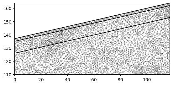
mesh = mt.createMesh(geom, quality=34.3, area=3, smooth=[1, 10])
ax, _ = pg.show(mesh)

• 
• 

Next we define geophone positions and a measurement scheme, which consists of shot and receiver indices.

numberGeophones = 48
sensors = np.linspace(0., 117.5, numberGeophones)
scheme = tt.createRAData(sensors, shotDistance=3)

# Adapt sensor positions to slope
slope = (164 - 137) / 117.5
pos = np.array(scheme.sensors())
for x in pos[:, 0]:
    i = np.where(pos[:, 0] == x)
    new_y = x * slope + 137
    pos[i, 1] = new_y

scheme.setSensors(pos)

Synthetic data generation

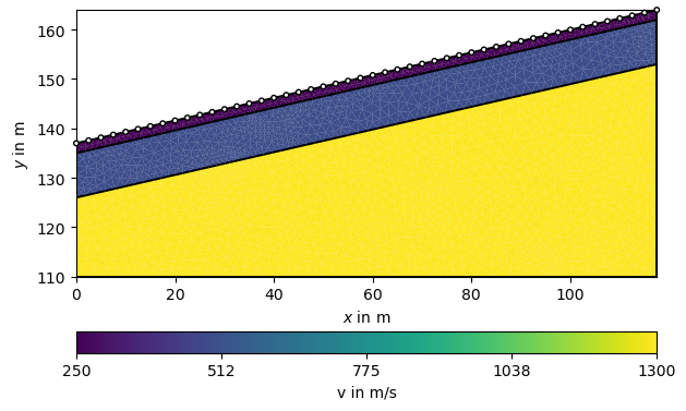
Now we initialize the TravelTime manager and asssign P-wave velocities to the layers. To this end, we create a map from cell markers 0 through 3 to velocities (in m/s) and generate a velocity vector. To check whether the model looks correct, we plot it along with the sensor positions.

vp = np.array(mesh.cellMarkers())
vp[vp == 1] = 250
vp[vp == 2] = 500
vp[vp == 3] = 1300

ax, _ = pg.show(mesh, vp, colorBar=True, logScale=False, label='v in m/s')
pg.viewer.mpl.drawSensors(ax, scheme.sensors(), diam=1.0,
                         facecolor='white', edgecolor='black')

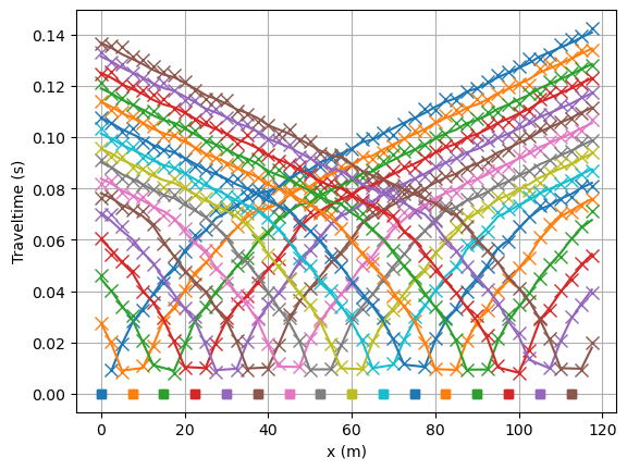
We use this model to create noisified synthetic data and look at the traveltime data matrix. Note, we force a specific noise seed as we want reproducable results for testing purposes.

data = tt.simulate(slowness=1.0 / vp, scheme=scheme, mesh=mesh,
                   noiseLevel=0.001, noiseAbs=0.001, seed=1337, verbose=True)
tt.show(data)

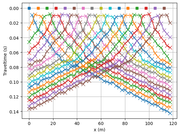
min/max t: 0.008790995543598544 0.14104424199242233

Inversion

Now we invert the synthetic data. We need a new independent mesh without information about the layered structure. This mesh can be created manual or guessd automatic from the data sensor positions (in this example). We tune the maximum cell size in the parametric domain to 15m²

mgr = tt.TravelTimeManager(data)
vest = mgr.invert(secNodes=2, paraMaxCellSize=15.0,
                  maxIter=10, verbose=True)
np.testing.assert_array_less(mgr.inv.inv.chi2(), 1.1)

fop: <pygimli.physics.traveltime.modelling.TravelTimeDijkstraModelling object at 0x172a97f10>
Data transformation: Identity transform
Model transformation: Logarithmic transform
min/max (data): 0.0079/0.14
min/max (error): 0.8%/12.81%
min/max (start model): 2.0e-04/0.002
--------------------------------------------------------------------------------
inv.iter 0 ... chi² =  635.23
--------------------------------------------------------------------------------
inv.iter 1 ... chi² =    3.07 (dPhi = 99.43%) lam: 20.0
--------------------------------------------------------------------------------
inv.iter 2 ... chi² =    1.66 (dPhi = 41.66%) lam: 20.0
--------------------------------------------------------------------------------
inv.iter 3 ... chi² =    1.24 (dPhi = 19.40%) lam: 20.0
--------------------------------------------------------------------------------
inv.iter 4 ... chi² =    1.01 (dPhi = 13.37%) lam: 20.0
--------------------------------------------------------------------------------
inv.iter 5 ... chi² =    0.85 (dPhi = 10.62%) lam: 20.0


################################################################################
#                  Abort criterion reached: chi² <= 1 (0.85)                   #
################################################################################

numpy.testing.assert_array_less

The manager also holds the method showResult that is used to plot the result. Note that only covered cells are shown by default. For comparison we plot the geometry on top.

ax, _ = mgr.showResult(cMin=min(vp), cMax=max(vp), logScale=False)
ax, _ = pg.show(geom, ax=ax, fillRegion=False, regionMarker=False)

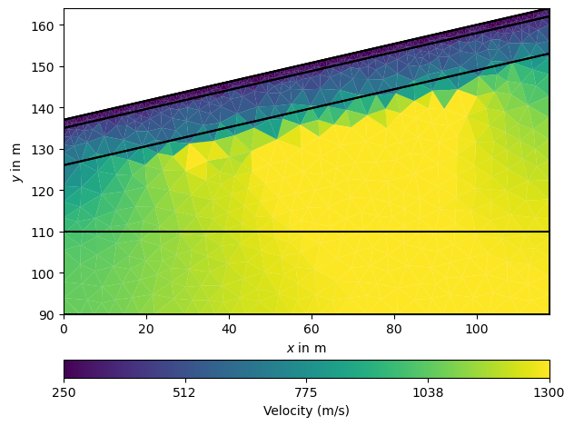
Note that internally the following is called

ax, _ = pg.show(ra.mesh, vest, label="Velocity [m/s]", **kwargs)

It is always important to have a look at the data fit.

mgr.showFit(firstPicks=True)

Note

Takeaway message

A default data inversion with checking of the data consists of only few lines. Check out Field data inversion (“Koenigsee”).