Fitting SIP signatures

This example highlights some of the capabilities of pyGimli to analyze spectral induced polarization (SIP) signatures.

Author: Maximilian Weigand, University of Bonn

Import pyGIMLi and related stuff for SIP Spectra

from pygimli.physics.SIP import SIPSpectrum, modelColeColeRho
import numpy as np
import pygimli as pg

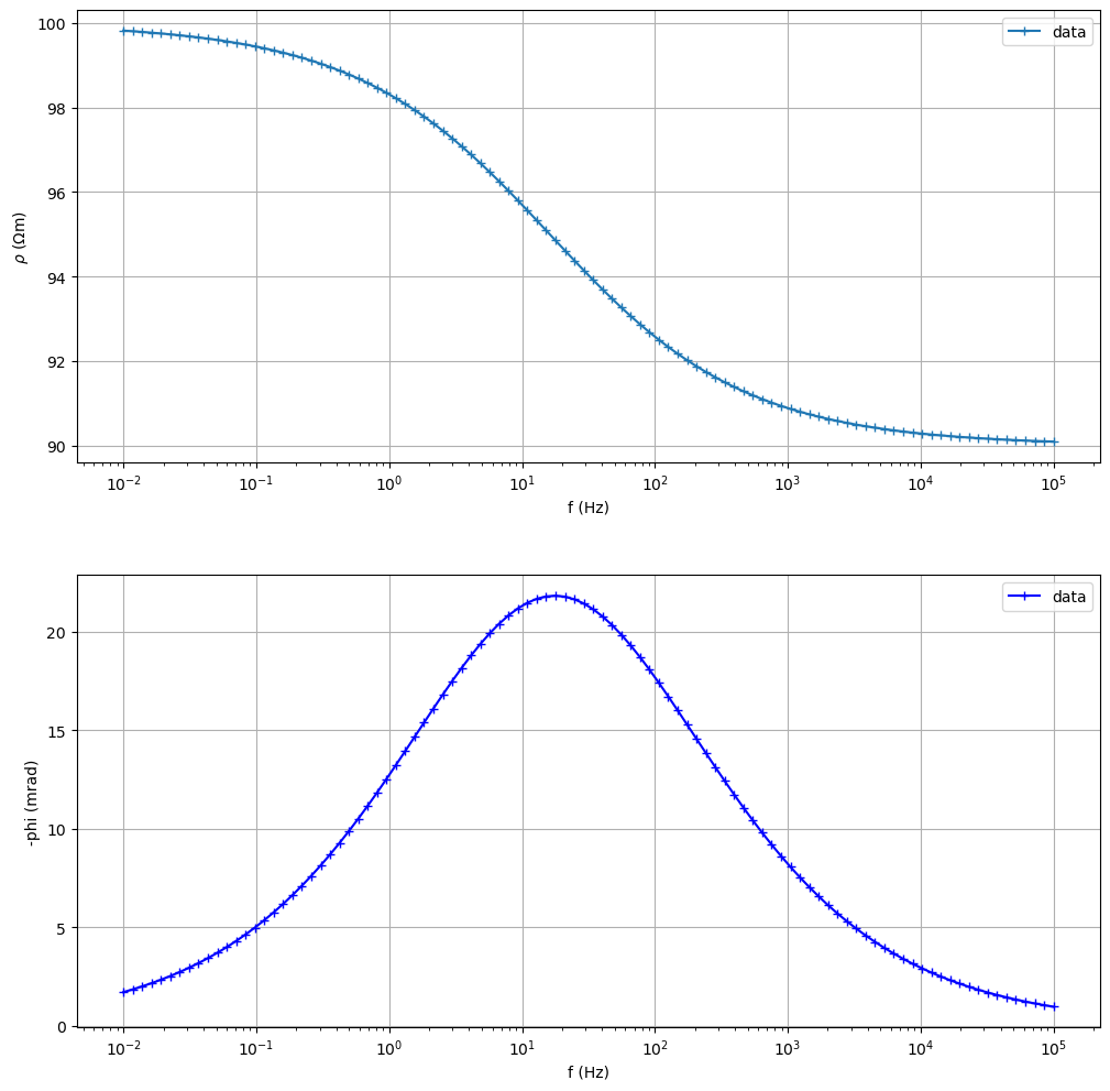
1. Generate synthetic data with a Double-Cole-Cole Model and initialize a SIPSpectrum object

f = np.logspace(-2, 5, 100)
Z1 = modelColeColeRho(f, rho=1, m=0.1, tau=0.5, c=0.5)
Z2 = modelColeColeRho(f, rho=1, m=0.25, tau=1e-6, c=1.0)

rho0 = 100 # (Ohm m)
Z = rho0 * (Z1 + Z2)

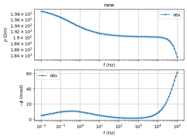
sip = SIPSpectrum(f=f, amp=np.abs(Z), phi=-np.angle(Z))
# Note the minus sign for the phases: we need to provide -phase[rad]

sip.showData()
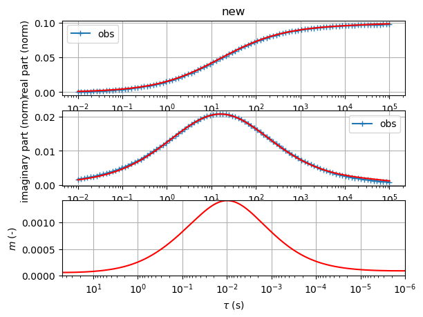
sip.showDataKK()  # check Kramers-Kronig relations

• 
• 

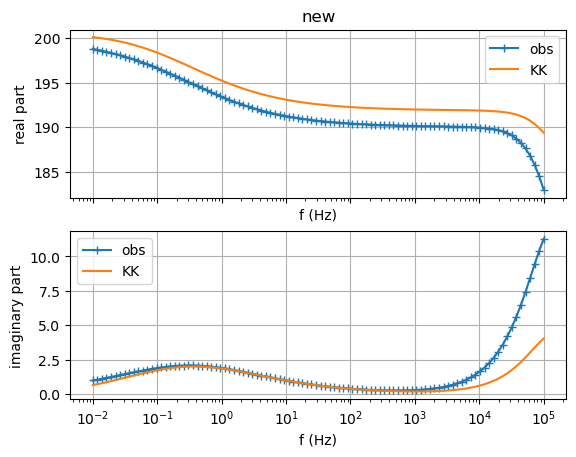
(<Figure size 640x480 with 2 Axes>, array([<Axes: title={'center': 'new'}, xlabel='f (Hz)', ylabel='real part'>,
       <Axes: xlabel='f (Hz)', ylabel='imaginary part'>], dtype=object))

2. Fit a Cole-Cole model from synthetic data

Z = modelColeColeRho(f, rho=100, m=0.1, tau=0.01, c=0.5)
# TODO data need some noise

sip = SIPSpectrum(f=f, amp=np.abs(Z), phi=-np.angle(Z))
sip.fitColeCole(useCond=False, verbose=False)  # works for both rho and sigma models
sip.showAll()

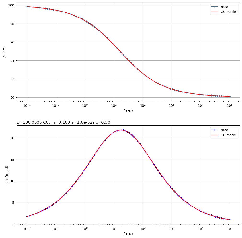
(<Figure size 1200x1200 with 2 Axes>, array([<Axes: xlabel='f (Hz)', ylabel='$\\rho$ ($\\Omega$m)'>,
       <Axes: title={'left': '$\\rho$=100.0000 CC: m=0.100 $\\tau$=1.0e-02s c=0.50 '}, xlabel='f (Hz)', ylabel='-phi (mrad)'>],
      dtype=object))

3. Fit a double Cole-Cole model

f = np.logspace(-2, 5, 100)
Z1 = modelColeColeRho(f, rho=1, m=0.1, tau=0.5, c=0.5)
Z2 = modelColeColeRho(f, rho=1, m=0.25, tau=1e-6, c=1.0)

rho0 = 100 #(Ohm m)
Z = rho0 * (Z1 + Z2)

# TODO data need some noise
sip = SIPSpectrum(f=f, amp=np.abs(Z), phi=-np.angle(Z))
sip.fitCCEM(verbose=False) # fit an SIP Cole-Cole term and an EM term (also Cole-Cole)
sip.showAll()

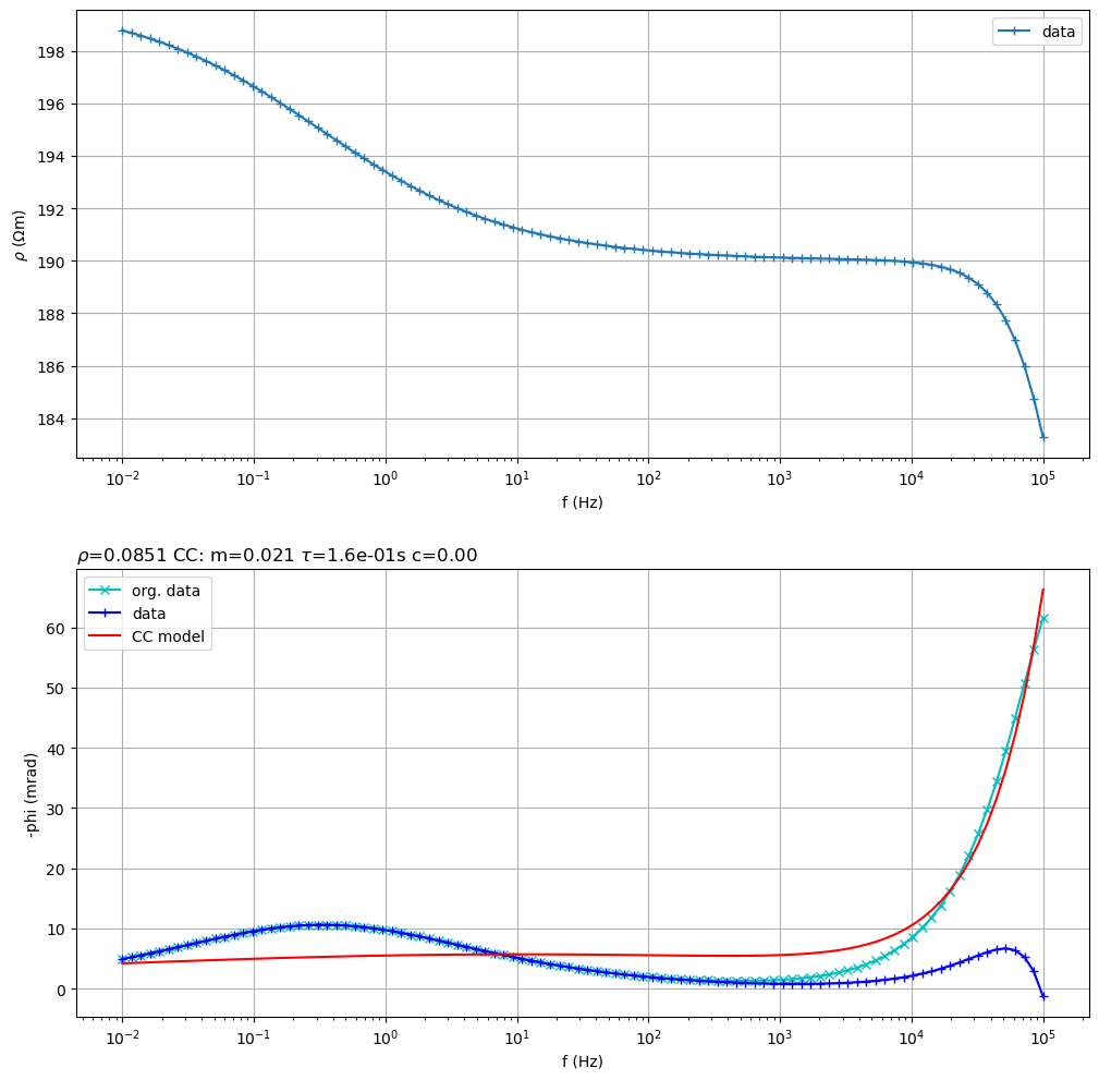
(<Figure size 1200x1200 with 2 Axes>, array([<Axes: xlabel='f (Hz)', ylabel='$\\rho$ ($\\Omega$m)'>,
       <Axes: title={'left': '$\\rho$=0.0851 CC: m=0.021 $\\tau$=1.6e-01s c=0.00 '}, xlabel='f (Hz)', ylabel='-phi (mrad)'>],
      dtype=object))

3. Fit a Cole-Cole model to

f = np.logspace(-2, 5, 100)
Z = modelColeColeRho(f, rho=100, m=0.1, tau=0.01, c=0.5)
sip = SIPSpectrum(f=f, amp=np.abs(Z), phi=-np.angle(Z))

sip.showAll()
sip.fitDebyeModel(new=True, showFit=True)
pg.wait()

• 
• 

ARMS= 0.0003210420209255598 RRMS= 0.3292375674156702

Note

This tutorial was kindly contributed by Maximilian Weigand (University of Bonn). If you also want to contribute an interesting example, check out our contribution guidelines https://www.pygimli.org/contrib.html.