Note
Go to the end to download the full example code.
Computing resolution properties#
This example demonstrates how block and smooth TEM modelling is done and how to access resolution matrices and kernels.
We import the necessary libraries
import numpy as np
import matplotlib.pyplot as plt
import pygimli as pg
from pygimli.physics import em
from pygimli.viewer.mpl import drawModel1D
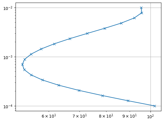
Next, we define a time vector from 100µs to 10ms and assume a loop of 100x100m. We use the TDEMBlockModelling operator to generate synthetic data for a three-layer case and plot it. Note that the output is apparent resistivity. We could now setup a Marquard-type block inversion as done in the VES example.
Instead, we want to do a smooth (Occam) style inversion where the layer thicknesses are known. For this, we use the TDEMSmoothModelling operator and logarithmic transforms for both model and data.
302.43843861107877
fop: <pygimli.physics.em.tdem.TDEMSmoothModelling object at 0x34c0d1710>
Data transformation: Logarithmic transform
Model transformation: Logarithmic transform
min/max (data): 52.5/102
min/max (error): 3%/3%
min/max (start model): 68.23/68.23
--------------------------------------------------------------------------------
inv.iter 0 ... chi² =   55.52
--------------------------------------------------------------------------------
inv.iter 1 ... chi² =   23.79 (dPhi = 56.76%) lam: 20.0
--------------------------------------------------------------------------------
inv.iter 2 ... chi² =    8.46 (dPhi = 60.27%) lam: 20.0
--------------------------------------------------------------------------------
inv.iter 3 ... chi² =    0.41 (dPhi = 77.27%) lam: 20.0


################################################################################
#                  Abort criterion reached: chi² <= 1 (0.41)                   #
################################################################################
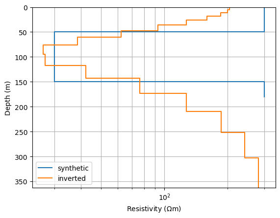
The inverted model is plotted along with the synthetic model, it resembles a smoothed image of it.
We are now interested in the resolution properties of the inverse problem. We call the function resolution matrix and obtain both the model resolution and the data resolution matrices. For only one, there are the functions modelResolutionMatrix and dataResolutionMatrix.
We display the model resolution matrix using imshow.
fig, ax = plt.subplots()
im = ax.imshow(RM, vmin=-0.3, vmax=0.3, cmap="RdBu_r")
ticks = np.arange(0, len(z), 2)
labels = [f"{zi:.0f}" for zi in z[ticks]]
ax.set_xticks(ticks)
ax.set_xticklabels(labels)
ax.set_yticks(ticks)
ax.set_yticklabels(labels)
cb = plt.colorbar(im)
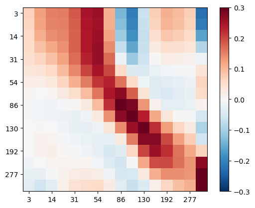
Except the last layer, the highest values occur on the main diagonal with maximum values at depths of about 100-200m. We can plot this formal resolution
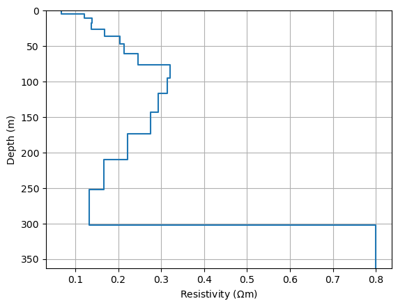
A single resolution kernel can be obtained by extracting a column of the matrix. For large-scale inverse problems, the model size might be too big to compute the whole matrix. One can then compute single resolution kernels by solving an inverse problem using modelResolutionKernel.
from pygimli.frameworks.resolution import modelResolutionKernel
fig, ax = plt.subplots()
nr = 10
drawModel1D(ax, plot="plot", thickness=thk, values=RM[:, nr], label="column")
knl = modelResolutionKernel(inv, nr)
drawModel1D(ax, plot="plot", thickness=thk, values=knl, label="kernel", ls="--")
ax.legend()
ax.hlines(z[nr], *ax.get_xlim())
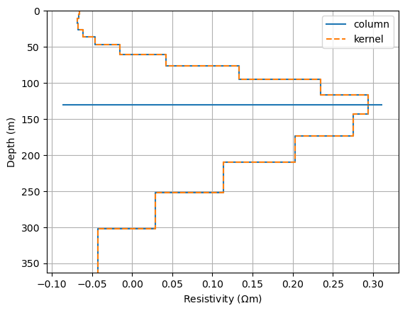
<matplotlib.collections.LineCollection object at 0x323d894c0>
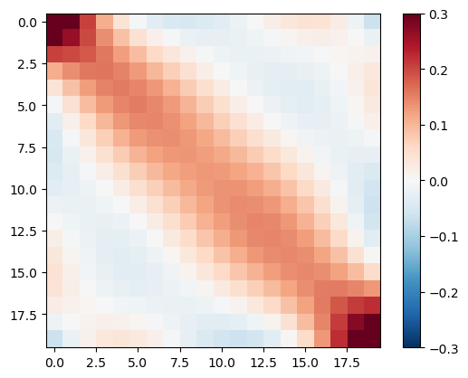
We also have a look at the data resolution matrix telling us about the inter-dependency and information content of the individual data.
im = plt.imshow(RD, vmin=-0.3, vmax=0.3, cmap="RdBu_r")
plt.colorbar(im)
<matplotlib.colorbar.Colorbar object at 0x340927470>
As expected, the neighboring time gates are highly correlated. The most important gates are the lowest and highest one as they define the first and last layers and cannot be replaced by others.
Total running time of the script: (0 minutes 28.891 seconds)